
|
Welcome to ShortScience.org! |


|
- ShortScience.org is a platform for post-publication discussion aiming to improve accessibility and reproducibility of research ideas.
- The website has 1584 public summaries, mostly in machine learning, written by the community and organized by paper, conference, and year.
- Reading summaries of papers is useful to obtain the perspective and insight of another reader, why they liked or disliked it, and their attempt to demystify complicated sections.
- Also, writing summaries is a good exercise to understand the content of a paper because you are forced to challenge your assumptions when explaining it.
- Finally, you can keep up to date with the flood of research by reading the latest summaries on our Twitter and Facebook pages.
Teaching Machines to Read and Comprehend
Hermann, Karl Moritz and Kociský, Tomás and Grefenstette, Edward and Espeholt, Lasse and Kay, Will and Suleyman, Mustafa and Blunsom, Phil
Neural Information Processing Systems Conference - 2015 via Local Bibsonomy
Keywords: dblp
Hermann, Karl Moritz and Kociský, Tomás and Grefenstette, Edward and Espeholt, Lasse and Kay, Will and Suleyman, Mustafa and Blunsom, Phil
Neural Information Processing Systems Conference - 2015 via Local Bibsonomy
Keywords: dblp


[link]
This paper deals with the formal question of machine reading. It proposes a novel methodology for automatic dataset building for machine reading model evaluation. To do so, the authors leverage on news resources that are equipped with a summary to generate a large number of questions about articles by replacing the named entities of it. Furthermore a attention enhanced LSTM inspired reading model is proposed and evaluated. The paper is well-written and clear, the originality seems to lie on two aspects. First, an original methodology of question answering dataset creation, where context-query-answer triples are automatically extracted from news feeds. Such proposition can be considered as important because it opens the way for large model learning and evaluation. The second contribution is the addition of an attention mechanism to an LSTM reading model. the empirical results seem to show relevant improvement with respect to an up-to-date list of machine reading models. Given the lack of an appropriate dataset, the author provides a new dataset which scraped CNN and Daily Mail, using both the full text and abstract summaries/bullet points. The dataset was then anonymised (i.e. entity names removed). Next the author presents a two novel Deep long-short term memory models which perform well on the Cloze query task.  |

Better-than-Demonstrator Imitation Learning via Automatically-Ranked Demonstrations
Daniel S. Brown and Wonjoon Goo and Scott Niekum
arXiv e-Print archive - 2019 via Local arXiv
Keywords: cs.LG, stat.ML
First published: 2019/07/09 (4 years ago)
Abstract: The performance of imitation learning is typically upper-bounded by the performance of the demonstrator. While recent empirical results demonstrate that ranked demonstrations allow for better-than-demonstrator performance, preferences over demonstrations may be difficult to obtain, and little is known theoretically about when such methods can be expected to successfully extrapolate beyond the performance of the demonstrator. To address these issues, we first contribute a sufficient condition for better-than-demonstrator imitation learning and provide theoretical results showing why preferences over demonstrations can better reduce reward function ambiguity when performing inverse reinforcement learning. Building on this theory, we introduce Disturbance-based Reward Extrapolation (D-REX), a ranking-based imitation learning method that injects noise into a policy learned through behavioral cloning to automatically generate ranked demonstrations. These ranked demonstrations are used to efficiently learn a reward function that can then be optimized using reinforcement learning. We empirically validate our approach on simulated robot and Atari imitation learning benchmarks and show that D-REX outperforms standard imitation learning approaches and can significantly surpass the performance of the demonstrator. D-REX is the first imitation learning approach to achieve significant extrapolation beyond the demonstrator's performance without additional side-information or supervision, such as rewards or human preferences. By generating rankings automatically, we show that preference-based inverse reinforcement learning can be applied in traditional imitation learning settings where only unlabeled demonstrations are available.
more
less
Daniel S. Brown and Wonjoon Goo and Scott Niekum
arXiv e-Print archive - 2019 via Local arXiv
Keywords: cs.LG, stat.ML
First published: 2019/07/09 (4 years ago)
Abstract: The performance of imitation learning is typically upper-bounded by the performance of the demonstrator. While recent empirical results demonstrate that ranked demonstrations allow for better-than-demonstrator performance, preferences over demonstrations may be difficult to obtain, and little is known theoretically about when such methods can be expected to successfully extrapolate beyond the performance of the demonstrator. To address these issues, we first contribute a sufficient condition for better-than-demonstrator imitation learning and provide theoretical results showing why preferences over demonstrations can better reduce reward function ambiguity when performing inverse reinforcement learning. Building on this theory, we introduce Disturbance-based Reward Extrapolation (D-REX), a ranking-based imitation learning method that injects noise into a policy learned through behavioral cloning to automatically generate ranked demonstrations. These ranked demonstrations are used to efficiently learn a reward function that can then be optimized using reinforcement learning. We empirically validate our approach on simulated robot and Atari imitation learning benchmarks and show that D-REX outperforms standard imitation learning approaches and can significantly surpass the performance of the demonstrator. D-REX is the first imitation learning approach to achieve significant extrapolation beyond the demonstrator's performance without additional side-information or supervision, such as rewards or human preferences. By generating rankings automatically, we show that preference-based inverse reinforcement learning can be applied in traditional imitation learning settings where only unlabeled demonstrations are available.
|
[link]
## General Framework Extends T-REX (see [summary](https://www.shortscience.org/paper?bibtexKey=journals/corr/1904.06387&a=muntermulehitch)) so that preferences (rankings) over demonstrations are generated automatically (back to the common IL/IRL setting where we only have access to a set of unlabeled demonstrations). Also derives some theoretical requirements and guarantees for better-than-demonstrator performance. ## Motivations * Preferences over demonstrations may be difficult to obtain in practice. * There is no theoretical understanding of the requirements that lead to outperforming demonstrator. ## Contributions * Theoretical results (with linear reward function) on when better-than-demonstrator performance is possible: 1- the demonstrator must be suboptimal (room for improvement, obviously), 2- the learned reward must be close enough to the reward that the demonstrator is suboptimally optimizing for (be able to accurately capture the intent of the demonstrator), 3- the learned policy (optimal wrt the learned reward) must be close enough to the optimal policy (wrt to the ground truth reward). Obviously if we have 2- and a good enough RL algorithm we should have 3-, so it might be interesting to see if one can derive a requirement from only 1- and 2- (and possibly a good enough RL algo). * Theoretical results (with linear reward function) showing that pairwise preferences over demonstrations reduce the error and ambiguity of the reward learning. They show that without rankings two policies might have equal performance under a learned reward (that makes expert's demonstrations optimal) but very different performance under the true reward (that makes the expert optimal everywhere). Indeed, the expert's demonstration may reveal very little information about the reward of (suboptimal or not) unseen regions which may hurt very much the generalizations (even with RL as it would try to generalize to new states under a totally wrong reward). They also show that pairwise preferences over trajectories effectively give half-space constraints on the feasible reward function domain and thus may decrease exponentially the reward function ambiguity. * Propose a practical way to generate as many ranked demos as desired. ## Additional Assumption Very mild, assumes that a Behavioral Cloning (BC) policy trained on the provided demonstrations is better than a uniform random policy. ## Disturbance-based Reward Extrapolation (D-REX)   They also show that the more noise added to the BC policy the lower the performance of the generated trajs. ## Results Pretty much like T-REX. |

Generating Images with Perceptual Similarity Metrics based on Deep Networks
Alexey Dosovitskiy and Thomas Brox
arXiv e-Print archive - 2016 via Local arXiv
Keywords: cs.LG, cs.CV, cs.NE
First published: 2016/02/08 (8 years ago)
Abstract: Image-generating machine learning models are typically trained with loss functions based on distance in the image space. This often leads to over-smoothed results. We propose a class of loss functions, which we call deep perceptual similarity metrics (DeePSiM), that mitigate this problem. Instead of computing distances in the image space, we compute distances between image features extracted by deep neural networks. This metric better reflects perceptually similarity of images and thus leads to better results. We show three applications: autoencoder training, a modification of a variational autoencoder, and inversion of deep convolutional networks. In all cases, the generated images look sharp and resemble natural images.
more
less
Alexey Dosovitskiy and Thomas Brox
arXiv e-Print archive - 2016 via Local arXiv
Keywords: cs.LG, cs.CV, cs.NE
First published: 2016/02/08 (8 years ago)
Abstract: Image-generating machine learning models are typically trained with loss functions based on distance in the image space. This often leads to over-smoothed results. We propose a class of loss functions, which we call deep perceptual similarity metrics (DeePSiM), that mitigate this problem. Instead of computing distances in the image space, we compute distances between image features extracted by deep neural networks. This metric better reflects perceptually similarity of images and thus leads to better results. We show three applications: autoencoder training, a modification of a variational autoencoder, and inversion of deep convolutional networks. In all cases, the generated images look sharp and resemble natural images.
|
[link]
* The authors define in this paper a special loss function (DeePSiM), mostly for autoencoders.
* Usually one would use a MSE of euclidean distance as the loss function for an autoencoder. But that loss function basically always leads to blurry reconstructed images.
* They add two new ingredients to the loss function, which results in significantly sharper looking images.
### How
* Their loss function has three components:
* Euclidean distance in image space (i.e. pixel distance between reconstructed image and original image, as usually used in autoencoders)
* Euclidean distance in feature space. Another pretrained neural net (e.g. VGG, AlexNet, ...) is used to extract features from the original and the reconstructed image. Then the euclidean distance between both vectors is measured.
* Adversarial loss, as usually used in GANs (generative adversarial networks). The autoencoder is here treated as the GAN-Generator. Then a second network, the GAN-Discriminator is introduced. They are trained in the typical GAN-fashion. The loss component for DeePSiM is the loss of the Discriminator. I.e. when reconstructing an image, the autoencoder would learn to reconstruct it in a way that lets the Discriminator believe that the image is real.
* Using the loss in feature space alone would not be enough as that tends to lead to overpronounced high frequency components in the image (i.e. too strong edges, corners, other artefacts).
* To decrease these high frequency components, a "natural image prior" is usually used. Other papers define some function by hand. This paper uses the adversarial loss for that (i.e. learns a good prior).
* Instead of training a full autoencoder (encoder + decoder) it is also possible to only train a decoder and feed features - e.g. extracted via AlexNet - into the decoder.
### Results
* Using the DeePSiM loss with a normal autoencoder results in sharp reconstructed images.
* Using the DeePSiM loss with a VAE to generate ILSVRC-2012 images results in sharp images, which are locally sound, but globally don't make sense. Simple euclidean distance loss results in blurry images.
* Using the DeePSiM loss when feeding only image space features (extracted via AlexNet) into the decoder leads to high quality reconstructions. Features from early layers will lead to more exact reconstructions.
* One can again feed extracted features into the network, but then take the reconstructed image, extract features of that image and feed them back into the network. When using DeePSiM, even after several iterations of that process the images still remain semantically similar, while their exact appearance changes (e.g. a dog's fur color might change, counts of visible objects change).
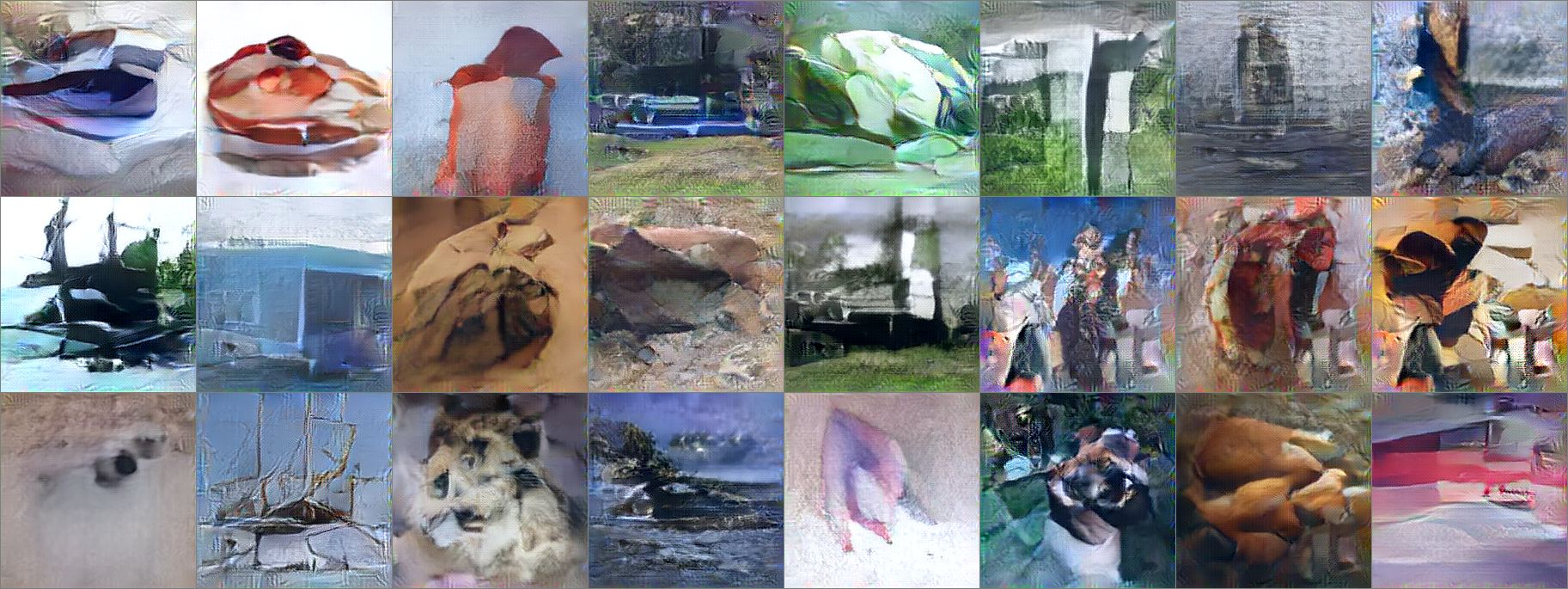
*Images generated with a VAE using DeePSiM loss.*
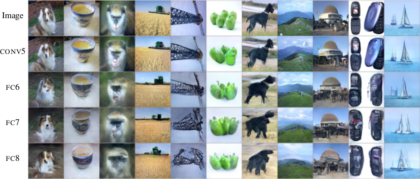
*Images reconstructed from features fed into the network. Different AlexNet layers (conv5 - fc8) were used to generate the features. Earlier layers allow more exact reconstruction.*
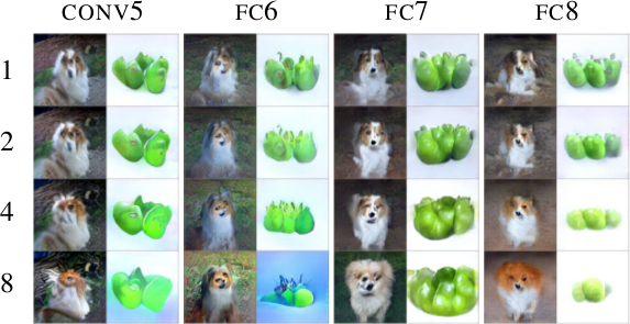
*First, images are reconstructed from features (AlexNet, layers conv5 - fc8 as columns). Then, features of the reconstructed images are fed back into the network. That is repeated up to 8 times (rows). Images stay semantically similar, but their appearance changes.*
--------------------
### Rough chapter-wise notes
* (1) Introduction
* Using a MSE of euclidean distances for image generation (e.g. autoencoders) often results in blurry images.
* They suggest a better loss function that cares about the existence of features, but not as much about their exact translation, rotation or other local statistics.
* Their loss function is based on distances in suitable feature spaces.
* They use ConvNets to generate those feature spaces, as these networks are sensitive towards important changes (e.g. edges) and insensitive towards unimportant changes (e.g. translation).
* However, naively using the ConvNet features does not yield good results, because the networks tend to project very different images onto the same feature vectors (i.e. they are contractive). That leads to artefacts in the generated images.
* Instead, they combine the feature based loss with GANs (adversarial loss). The adversarial loss decreases the negative effects of the feature loss ("natural image prior").
* (3) Model
* A typical choice for the loss function in image generation tasks (e.g. when using an autoencoders) would be squared euclidean/L2 loss or L1 loss.
* They suggest a new class of losses called "DeePSiM".
* We have a Generator `G`, a Discriminator `D`, a feature space creator `C` (takes an image, outputs a feature space for that image), one (or more) input images `x` and one (or more) target images `y`. Input and target image can be identical.
* The total DeePSiM loss is a weighted sum of three components:
* Feature loss: Squared euclidean distance between the feature spaces of (1) input after fed through G and (2) the target image, i.e. `||C(G(x))-C(y)||^2_2`.
* Adversarial loss: A discriminator is introduced to estimate the "fakeness" of images generated by the generator. The losses for D and G are the standard GAN losses.
* Pixel space loss: Classic squared euclidean distance (as commonly used in autoencoders). They found that this loss stabilized their adversarial training.
* The feature loss alone would create high frequency artefacts in the generated image, which is why a second loss ("natural image prior") is needed. The adversarial loss fulfills that role.
* Architectures
* Generator (G):
* They define different ones based on the task.
* They all use up-convolutions, which they implement by stacking two layers: (1) a linear upsampling layer, then (2) a normal convolutional layer.
* They use leaky ReLUs (alpha=0.3).
* Comparators (C):
* They use variations of AlexNet and Exemplar-CNN.
* They extract the features from different layers, depending on the experiment.
* Discriminator (D):
* 5 convolutions (with some striding; 7x7 then 5x5, afterwards 3x3), into average pooling, then dropout, then 2x linear, then 2-way softmax.
* Training details
* They use Adam with learning rate 0.0002 and normal momentums (0.9 and 0.999).
* They temporarily stop the discriminator training when it gets too good.
* Batch size was 64.
* 500k to 1000k batches per training.
* (4) Experiments
* Autoencoder
* Simple autoencoder with an 8x8x8 code layer between encoder and decoder (so actually more values than in the input image?!).
* Encoder has a few convolutions, decoder a few up-convolutions (linear upsampling + convolution).
* They train on STL-10 (96x96) and take random 64x64 crops.
* Using for C AlexNet tends to break small structural details, using Exempler-CNN breaks color details.
* The autoencoder with their loss tends to produce less blurry images than the common L2 and L1 based losses.
* Training an SVM on the 8x8x8 hidden layer performs significantly with their loss than L2/L1. That indicates potential for unsupervised learning.
* Variational Autoencoder
* They replace part of the standard VAE loss with their DeePSiM loss (keeping the KL divergence term).
* Everything else is just like in a standard VAE.
* Samples generated by a VAE with normal loss function look very blurry. Samples generated with their loss function look crisp and have locally sound statistics, but still (globally) don't really make any sense.
* Inverting AlexNet
* Assume the following variables:
* I: An image
* ConvNet: A convolutional network
* F: The features extracted by a ConvNet, i.e. ConvNet(I) (feaures in all layers, not just the last one)
* Then you can invert the representation of a network in two ways:
* (1) An inversion that takes an F and returns roughly the I that resulted in F (it's *not* key here that ConvNet(reconstructed I) returns the same F again).
* (2) An inversion that takes an F and projects it to *some* I so that ConvNet(I) returns roughly the same F again.
* Similar to the autoencoder cases, they define a decoder, but not encoder.
* They feed into the decoder a feature representation of an image. The features are extracted using AlexNet (they try the features from different layers).
* The decoder has to reconstruct the original image (i.e. inversion scenario 1). They use their DeePSiM loss during the training.
* The images can be reonstructed quite well from the last convolutional layer in AlexNet. Chosing the later fully connected layers results in more errors (specifially in the case of the very last layer).
* They also try their luck with the inversion scenario (2), but didn't succeed (as their loss function does not care about diversity).
* They iteratively encode and decode the same image multiple times (probably means: image -> features via AlexNet -> decode -> reconstructed image -> features via AlexNet -> decode -> ...). They observe, that the image does not get "destroyed", but rather changes semantically, e.g. three apples might turn to one after several steps.
* They interpolate between images. The interpolations are smooth.
|

The Shattered Gradients Problem: If resnets are the answer, then what is the question?
Balduzzi, David and Frean, Marcus and Leary, Lennox and Lewis, J. P. and Ma, Kurt Wan-Duo and McWilliams, Brian
International Conference on Machine Learning - 2017 via Local Bibsonomy
Keywords: dblp
Balduzzi, David and Frean, Marcus and Leary, Lennox and Lewis, J. P. and Ma, Kurt Wan-Duo and McWilliams, Brian
International Conference on Machine Learning - 2017 via Local Bibsonomy
Keywords: dblp
|
[link]
Imagine you make a neural network mapping a scalar to a scalar. After you initialise this network in the traditional way, randomly with some given variance, you could take the gradient of the input with respect to the output for all reasonable values (between about - and 3 because networks typically assume standardised inputs). As the value increases, different rectified linear units in the network will randomly switch on, drawing a random walk in the gradients; another name for which is brown noise.

However, do the same thing for deep networks, and any traditional initialisation you choose, and you'll see the random walk start to look like white noise. One intuition given in the paper is that as different rectifiers in the network switch off and on the input is taking a number of different paths though the network. The number of possible paths grows exponentially with the depth of the network, so as the input varies, the gradients become increasingly chaotic. **The explanations and derivations given in the paper are much better reasoned and thorough, please read those if you are interested**.
Why should we care about this? Because the authors take the recent nonlinearity [CReLU][] (output is concatenation of `relu(x)` and `relu(-x)`) and develop an initialisation that will avoid problems with gradient shattering. The initialisation is just to take your standard initialised weight matrix $\mathbf{W}$ and set the right half to be the negative of the left half ($\mathbf{W}_{\text{left}}$). As long as the input to the layer is also concatenated, the left half will be multiplied by `relu(x)` and the right by `relu(-x)`. Then:
$$
\mathbf{W}.\text{CReLU}(\mathbf{x}) = \begin{cases} \mathbf{W}_{\text{left}}\mathbf{x} & \text{ if } x > 0 \\ \mathbf{W}_{\text{left}}\mathbf{x} & \text{ if } x \leq 0\end{cases}
$$
Doing this allows them to train deep networks without skip connections, and they show results on CIFAR-10 with depths of up to 200 exceeding (slightly) a similar resnet.
[crelu]: https://arxiv.org/abs/1603.05201
|

Batch Normalization: Accelerating Deep Network Training by Reducing Internal Covariate Shift
Ioffe, Sergey and Szegedy, Christian
International Conference on Machine Learning - 2015 via Local Bibsonomy
Keywords: dblp
Ioffe, Sergey and Szegedy, Christian
International Conference on Machine Learning - 2015 via Local Bibsonomy
Keywords: dblp
|
[link]
The main contribution of this paper is introducing a new transformation that the authors call Batch Normalization (BN). The need for BN comes from the fact that during the training of deep neural networks (DNNs) the distribution of each layer’s input change. This phenomenon is called internal covariate shift (ICS).

#### What is BN?
Normalize each (scalar) feature independently with respect to the mean and variance of the mini batch. Scale and shift the normalized values with two new parameters (per activation) that will be learned. The BN consists of making normalization part of the model architecture.

#### What do we gain?
According to the author, the use of BN provides a great speed up in the training of DNNs. In particular, the gains are greater when it is combined with higher learning rates. In addition, BN works as a regularizer for the model which allows to use less dropout or less L2 normalization. Furthermore, since the distribution of the inputs is normalized, it also allows to use sigmoids as activation functions without the saturation problem.

#### What follows?
This seems to be specially promising for training recurrent neural networks (RNNs). The vanishing and exploding gradient problems \cite{journals/tnn/BengioSF94} have their origin in the iteration of transformation that scale up or down the activations in certain directions (eigenvectors). It seems that this regularization would be specially useful in this context since this would allow the gradient to flow more easily. When we unroll the RNNs, we usually have ultra deep networks.

#### Like
* Simple idea that seems to improve training.
* Makes training faster.
* Simple to implement. Probably.
* You can be less careful with initialization.

#### Dislike
* Does not work with stochastic gradient descent (minibatch size = 1).
* This could reduce the parallelism of the algorithm since now all the examples in a mini batch are tied.
* Results on ensemble of networks for ImageNet makes it harder to evaluate the relevance of BN by itself. (Although they do mention the performance of a single model).
|
