
|
Welcome to ShortScience.org! |


|
- ShortScience.org is a platform for post-publication discussion aiming to improve accessibility and reproducibility of research ideas.
- The website has 1584 public summaries, mostly in machine learning, written by the community and organized by paper, conference, and year.
- Reading summaries of papers is useful to obtain the perspective and insight of another reader, why they liked or disliked it, and their attempt to demystify complicated sections.
- Also, writing summaries is a good exercise to understand the content of a paper because you are forced to challenge your assumptions when explaining it.
- Finally, you can keep up to date with the flood of research by reading the latest summaries on our Twitter and Facebook pages.
Teaching Machines to Read and Comprehend
Hermann, Karl Moritz and Kociský, Tomás and Grefenstette, Edward and Espeholt, Lasse and Kay, Will and Suleyman, Mustafa and Blunsom, Phil
Neural Information Processing Systems Conference - 2015 via Local Bibsonomy
Keywords: dblp
Hermann, Karl Moritz and Kociský, Tomás and Grefenstette, Edward and Espeholt, Lasse and Kay, Will and Suleyman, Mustafa and Blunsom, Phil
Neural Information Processing Systems Conference - 2015 via Local Bibsonomy
Keywords: dblp


[link]
This paper deals with the formal question of machine reading. It proposes a novel methodology for automatic dataset building for machine reading model evaluation. To do so, the authors leverage on news resources that are equipped with a summary to generate a large number of questions about articles by replacing the named entities of it. Furthermore a attention enhanced LSTM inspired reading model is proposed and evaluated. The paper is well-written and clear, the originality seems to lie on two aspects. First, an original methodology of question answering dataset creation, where context-query-answer triples are automatically extracted from news feeds. Such proposition can be considered as important because it opens the way for large model learning and evaluation. The second contribution is the addition of an attention mechanism to an LSTM reading model. the empirical results seem to show relevant improvement with respect to an up-to-date list of machine reading models. Given the lack of an appropriate dataset, the author provides a new dataset which scraped CNN and Daily Mail, using both the full text and abstract summaries/bullet points. The dataset was then anonymised (i.e. entity names removed). Next the author presents a two novel Deep long-short term memory models which perform well on the Cloze query task.  |

Batch Normalization: Accelerating Deep Network Training by Reducing Internal Covariate Shift
Ioffe, Sergey and Szegedy, Christian
International Conference on Machine Learning - 2015 via Local Bibsonomy
Keywords: dblp
Ioffe, Sergey and Szegedy, Christian
International Conference on Machine Learning - 2015 via Local Bibsonomy
Keywords: dblp
|
[link]
The main contribution of this paper is introducing a new transformation that the authors call Batch Normalization (BN). The need for BN comes from the fact that during the training of deep neural networks (DNNs) the distribution of each layer’s input change. This phenomenon is called internal covariate shift (ICS).

#### What is BN?
Normalize each (scalar) feature independently with respect to the mean and variance of the mini batch. Scale and shift the normalized values with two new parameters (per activation) that will be learned. The BN consists of making normalization part of the model architecture.

#### What do we gain?
According to the author, the use of BN provides a great speed up in the training of DNNs. In particular, the gains are greater when it is combined with higher learning rates. In addition, BN works as a regularizer for the model which allows to use less dropout or less L2 normalization. Furthermore, since the distribution of the inputs is normalized, it also allows to use sigmoids as activation functions without the saturation problem.

#### What follows?
This seems to be specially promising for training recurrent neural networks (RNNs). The vanishing and exploding gradient problems \cite{journals/tnn/BengioSF94} have their origin in the iteration of transformation that scale up or down the activations in certain directions (eigenvectors). It seems that this regularization would be specially useful in this context since this would allow the gradient to flow more easily. When we unroll the RNNs, we usually have ultra deep networks.

#### Like
* Simple idea that seems to improve training.
* Makes training faster.
* Simple to implement. Probably.
* You can be less careful with initialization.

#### Dislike
* Does not work with stochastic gradient descent (minibatch size = 1).
* This could reduce the parallelism of the algorithm since now all the examples in a mini batch are tied.
* Results on ensemble of networks for ImageNet makes it harder to evaluate the relevance of BN by itself. (Although they do mention the performance of a single model).
|

Generating Images with Perceptual Similarity Metrics based on Deep Networks
Alexey Dosovitskiy and Thomas Brox
arXiv e-Print archive - 2016 via Local arXiv
Keywords: cs.LG, cs.CV, cs.NE
First published: 2016/02/08 (8 years ago)
Abstract: Image-generating machine learning models are typically trained with loss functions based on distance in the image space. This often leads to over-smoothed results. We propose a class of loss functions, which we call deep perceptual similarity metrics (DeePSiM), that mitigate this problem. Instead of computing distances in the image space, we compute distances between image features extracted by deep neural networks. This metric better reflects perceptually similarity of images and thus leads to better results. We show three applications: autoencoder training, a modification of a variational autoencoder, and inversion of deep convolutional networks. In all cases, the generated images look sharp and resemble natural images.
more
less
Alexey Dosovitskiy and Thomas Brox
arXiv e-Print archive - 2016 via Local arXiv
Keywords: cs.LG, cs.CV, cs.NE
First published: 2016/02/08 (8 years ago)
Abstract: Image-generating machine learning models are typically trained with loss functions based on distance in the image space. This often leads to over-smoothed results. We propose a class of loss functions, which we call deep perceptual similarity metrics (DeePSiM), that mitigate this problem. Instead of computing distances in the image space, we compute distances between image features extracted by deep neural networks. This metric better reflects perceptually similarity of images and thus leads to better results. We show three applications: autoencoder training, a modification of a variational autoencoder, and inversion of deep convolutional networks. In all cases, the generated images look sharp and resemble natural images.
|
[link]
* The authors define in this paper a special loss function (DeePSiM), mostly for autoencoders.
* Usually one would use a MSE of euclidean distance as the loss function for an autoencoder. But that loss function basically always leads to blurry reconstructed images.
* They add two new ingredients to the loss function, which results in significantly sharper looking images.
### How
* Their loss function has three components:
* Euclidean distance in image space (i.e. pixel distance between reconstructed image and original image, as usually used in autoencoders)
* Euclidean distance in feature space. Another pretrained neural net (e.g. VGG, AlexNet, ...) is used to extract features from the original and the reconstructed image. Then the euclidean distance between both vectors is measured.
* Adversarial loss, as usually used in GANs (generative adversarial networks). The autoencoder is here treated as the GAN-Generator. Then a second network, the GAN-Discriminator is introduced. They are trained in the typical GAN-fashion. The loss component for DeePSiM is the loss of the Discriminator. I.e. when reconstructing an image, the autoencoder would learn to reconstruct it in a way that lets the Discriminator believe that the image is real.
* Using the loss in feature space alone would not be enough as that tends to lead to overpronounced high frequency components in the image (i.e. too strong edges, corners, other artefacts).
* To decrease these high frequency components, a "natural image prior" is usually used. Other papers define some function by hand. This paper uses the adversarial loss for that (i.e. learns a good prior).
* Instead of training a full autoencoder (encoder + decoder) it is also possible to only train a decoder and feed features - e.g. extracted via AlexNet - into the decoder.
### Results
* Using the DeePSiM loss with a normal autoencoder results in sharp reconstructed images.
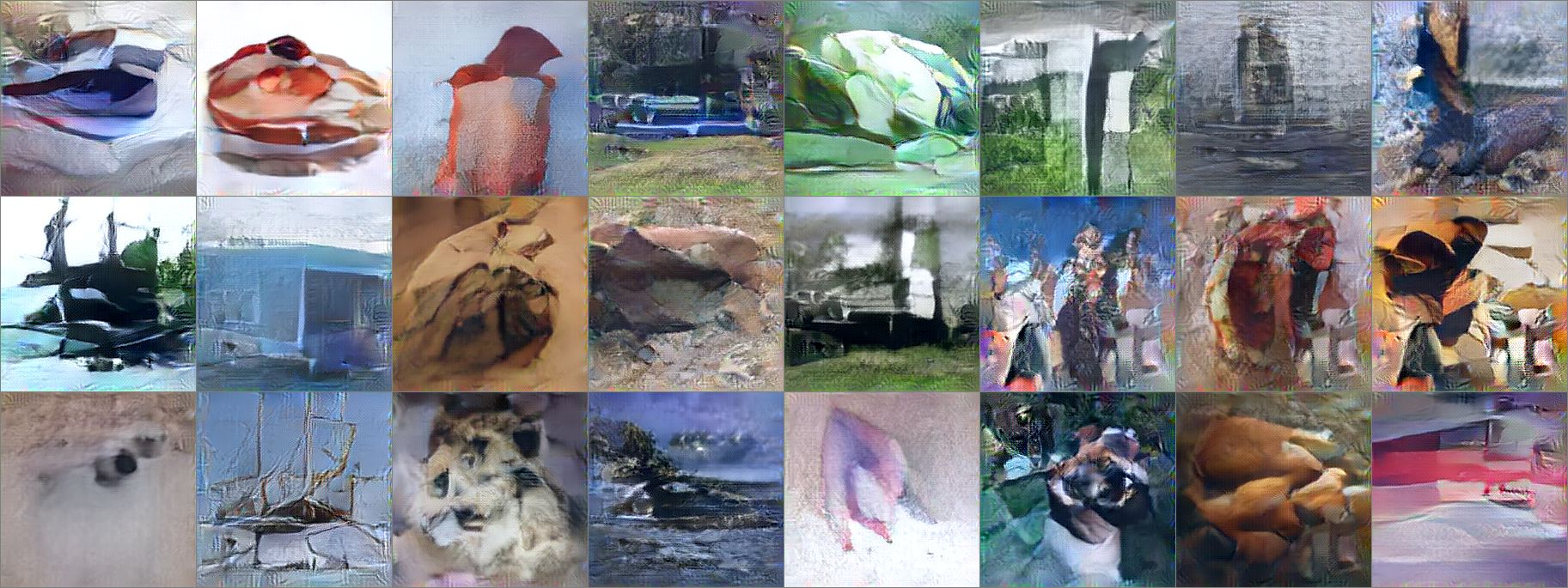
* Using the DeePSiM loss with a VAE to generate ILSVRC-2012 images results in sharp images, which are locally sound, but globally don't make sense. Simple euclidean distance loss results in blurry images.
* Using the DeePSiM loss when feeding only image space features (extracted via AlexNet) into the decoder leads to high quality reconstructions. Features from early layers will lead to more exact reconstructions.
* One can again feed extracted features into the network, but then take the reconstructed image, extract features of that image and feed them back into the network. When using DeePSiM, even after several iterations of that process the images still remain semantically similar, while their exact appearance changes (e.g. a dog's fur color might change, counts of visible objects change).
*Images generated with a VAE using DeePSiM loss.*
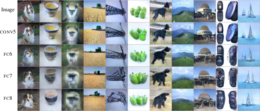
*Images reconstructed from features fed into the network. Different AlexNet layers (conv5 - fc8) were used to generate the features. Earlier layers allow more exact reconstruction.*
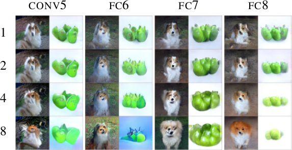
*First, images are reconstructed from features (AlexNet, layers conv5 - fc8 as columns). Then, features of the reconstructed images are fed back into the network. That is repeated up to 8 times (rows). Images stay semantically similar, but their appearance changes.*
--------------------
### Rough chapter-wise notes
* (1) Introduction
* Using a MSE of euclidean distances for image generation (e.g. autoencoders) often results in blurry images.
* They suggest a better loss function that cares about the existence of features, but not as much about their exact translation, rotation or other local statistics.
* Their loss function is based on distances in suitable feature spaces.
* They use ConvNets to generate those feature spaces, as these networks are sensitive towards important changes (e.g. edges) and insensitive towards unimportant changes (e.g. translation).
* However, naively using the ConvNet features does not yield good results, because the networks tend to project very different images onto the same feature vectors (i.e. they are contractive). That leads to artefacts in the generated images.
* Instead, they combine the feature based loss with GANs (adversarial loss). The adversarial loss decreases the negative effects of the feature loss ("natural image prior").
* (3) Model
* A typical choice for the loss function in image generation tasks (e.g. when using an autoencoders) would be squared euclidean/L2 loss or L1 loss.
* They suggest a new class of losses called "DeePSiM".
* We have a Generator `G`, a Discriminator `D`, a feature space creator `C` (takes an image, outputs a feature space for that image), one (or more) input images `x` and one (or more) target images `y`. Input and target image can be identical.
* The total DeePSiM loss is a weighted sum of three components:
* Feature loss: Squared euclidean distance between the feature spaces of (1) input after fed through G and (2) the target image, i.e. `||C(G(x))-C(y)||^2_2`.
* Adversarial loss: A discriminator is introduced to estimate the "fakeness" of images generated by the generator. The losses for D and G are the standard GAN losses.
* Pixel space loss: Classic squared euclidean distance (as commonly used in autoencoders). They found that this loss stabilized their adversarial training.
* The feature loss alone would create high frequency artefacts in the generated image, which is why a second loss ("natural image prior") is needed. The adversarial loss fulfills that role.
* Architectures
* Generator (G):
* They define different ones based on the task.
* They all use up-convolutions, which they implement by stacking two layers: (1) a linear upsampling layer, then (2) a normal convolutional layer.
* They use leaky ReLUs (alpha=0.3).
* Comparators (C):
* They use variations of AlexNet and Exemplar-CNN.
* They extract the features from different layers, depending on the experiment.
* Discriminator (D):
* 5 convolutions (with some striding; 7x7 then 5x5, afterwards 3x3), into average pooling, then dropout, then 2x linear, then 2-way softmax.
* Training details
* They use Adam with learning rate 0.0002 and normal momentums (0.9 and 0.999).
* They temporarily stop the discriminator training when it gets too good.
* Batch size was 64.
* 500k to 1000k batches per training.
* (4) Experiments
* Autoencoder
* Simple autoencoder with an 8x8x8 code layer between encoder and decoder (so actually more values than in the input image?!).
* Encoder has a few convolutions, decoder a few up-convolutions (linear upsampling + convolution).
* They train on STL-10 (96x96) and take random 64x64 crops.
* Using for C AlexNet tends to break small structural details, using Exempler-CNN breaks color details.
* The autoencoder with their loss tends to produce less blurry images than the common L2 and L1 based losses.
* Training an SVM on the 8x8x8 hidden layer performs significantly with their loss than L2/L1. That indicates potential for unsupervised learning.
* Variational Autoencoder
* They replace part of the standard VAE loss with their DeePSiM loss (keeping the KL divergence term).
* Everything else is just like in a standard VAE.
* Samples generated by a VAE with normal loss function look very blurry. Samples generated with their loss function look crisp and have locally sound statistics, but still (globally) don't really make any sense.
* Inverting AlexNet
* Assume the following variables:
* I: An image
* ConvNet: A convolutional network
* F: The features extracted by a ConvNet, i.e. ConvNet(I) (feaures in all layers, not just the last one)
* Then you can invert the representation of a network in two ways:
* (1) An inversion that takes an F and returns roughly the I that resulted in F (it's *not* key here that ConvNet(reconstructed I) returns the same F again).
* (2) An inversion that takes an F and projects it to *some* I so that ConvNet(I) returns roughly the same F again.
* Similar to the autoencoder cases, they define a decoder, but not encoder.
* They feed into the decoder a feature representation of an image. The features are extracted using AlexNet (they try the features from different layers).
* The decoder has to reconstruct the original image (i.e. inversion scenario 1). They use their DeePSiM loss during the training.
* The images can be reonstructed quite well from the last convolutional layer in AlexNet. Chosing the later fully connected layers results in more errors (specifially in the case of the very last layer).
* They also try their luck with the inversion scenario (2), but didn't succeed (as their loss function does not care about diversity).
* They iteratively encode and decode the same image multiple times (probably means: image -> features via AlexNet -> decode -> reconstructed image -> features via AlexNet -> decode -> ...). They observe, that the image does not get "destroyed", but rather changes semantically, e.g. three apples might turn to one after several steps.
* They interpolate between images. The interpolations are smooth.
|

Generative Adversarial Nets
Goodfellow, Ian J. and Pouget-Abadie, Jean and Mirza, Mehdi and Xu, Bing and Warde-Farley, David and Ozair, Sherjil and Courville, Aaron C. and Bengio, Yoshua
Neural Information Processing Systems Conference - 2014 via Local Bibsonomy
Keywords: dblp
Goodfellow, Ian J. and Pouget-Abadie, Jean and Mirza, Mehdi and Xu, Bing and Warde-Farley, David and Ozair, Sherjil and Courville, Aaron C. and Bengio, Yoshua
Neural Information Processing Systems Conference - 2014 via Local Bibsonomy
Keywords: dblp
|
[link]
* GANs are based on adversarial training.
* Adversarial training is a basic technique to train generative models (so here primarily models that create new images).
* In an adversarial training one model (G, Generator) generates things (e.g. images). Another model (D, discriminator) sees real things (e.g. real images) as well as fake things (e.g. images from G) and has to learn how to differentiate the two.
* Neural Networks are models that can be trained in an adversarial way (and are the only models discussed here).
### How
* G is a simple neural net (e.g. just one fully connected hidden layer). It takes a vector as input (e.g. 100 dimensions) and produces an image as output.
* D is a simple neural net (e.g. just one fully connected hidden layer). It takes an image as input and produces a quality rating as output (0-1, so sigmoid).
* You need a training set of things to be generated, e.g. images of human faces.
* Let the batch size be B.
* G is trained the following way:
* Create B vectors of 100 random values each, e.g. sampled uniformly from [-1, +1]. (Number of values per components depends on the chosen input size of G.)
* Feed forward the vectors through G to create new images.
* Feed forward the images through D to create ratings.
* Use a cross entropy loss on these ratings. All of these (fake) images should be viewed as label=0 by D. If D gives them label=1, the error will be low (G did a good job).
* Perform a backward pass of the errors through D (without training D). That generates gradients/errors per image and pixel.
* Perform a backward pass of these errors through G to train G.
* D is trained the following way:
* Create B/2 images using G (again, B/2 random vectors, feed forward through G).
* Chose B/2 images from the training set. Real images get label=1.
* Merge the fake and real images to one batch. Fake images get label=0.
* Feed forward the batch through D.
* Measure the error using cross entropy.
* Perform a backward pass with the error through D.
* Train G for one batch, then D for one (or more) batches. Sometimes D can be too slow to catch up with D, then you need more iterations of D per batch of G.
### Results
* Good looking images MNIST-numbers and human faces. (Grayscale, rather homogeneous datasets.)
* Not so good looking images of CIFAR-10. (Color, rather heterogeneous datasets.)

*Faces generated by MLP GANs. (Rightmost column shows examples from the training set.)*
-------------------------
### Rough chapter-wise notes
* Introduction
* Discriminative models performed well so far, generative models not so much.
* Their suggested new architecture involves a generator and a discriminator.
* The generator learns to create content (e.g. images), the discriminator learns to differentiate between real content and generated content.
* Analogy: Generator produces counterfeit art, discriminator's job is to judge whether a piece of art is a counterfeit.
* This principle could be used with many techniques, but they use neural nets (MLPs) for both the generator as well as the discriminator.
* Adversarial Nets
* They have a Generator G (simple neural net)
* G takes a random vector as input (e.g. vector of 100 random values between -1 and +1).
* G creates an image as output.
* They have a Discriminator D (simple neural net)
* D takes an image as input (can be real or generated by G).
* D creates a rating as output (quality, i.e. a value between 0 and 1, where 0 means "probably fake").
* Outputs from G are fed into D. The result can then be backpropagated through D and then G. G is trained to maximize log(D(image)), so to create a high value of D(image).
* D is trained to produce only 1s for images from G.
* Both are trained simultaneously, i.e. one batch for G, then one batch for D, then one batch for G...
* D can also be trained multiple times in a row. That allows it to catch up with G.
* Theoretical Results
* Let
* pd(x): Probability that image `x` appears in the training set.
* pg(x): Probability that image `x` appears in the images generated by G.
* If G is now fixed then the best possible D classifies according to: `D(x) = pd(x) / (pd(x) + pg(x))`
* It is proofable that there is only one global optimum for GANs, which is reached when G perfectly replicates the training set probability distribution. (Assuming unlimited capacity of the models and unlimited training time.)
* It is proofable that G and D will converge to the global optimum, so long as D gets enough steps per training iteration to model the distribution generated by G. (Again, assuming unlimited capacity/time.)
* Note that these things are proofed for the general principle for GANs. Implementing GANs with neural nets can then introduce problems typical for neural nets (e.g. getting stuck in saddle points).
* Experiments
* They tested on MNIST, Toronto Face Database (TFD) and CIFAR-10.
* They used MLPs for G and D.
* G contained ReLUs and Sigmoids.
* D contained Maxouts.
* D had Dropout, G didn't.
* They use a Parzen Window Estimate aka KDE (sigma obtained via cross validation) to estimate the quality of their images.
* They note that KDE is not really a great technique for such high dimensional spaces, but its the only one known.
* Results on MNIST and TDF are great. (Note: both grayscale)
* CIFAR-10 seems to match more the texture but not really the structure.
* Noise is noticeable in CIFAR-10 (a bit in TFD too). Comes from MLPs (no convolutions).
* Their KDE score for MNIST and TFD is competitive or better than other approaches.
* Advantages and Disadvantages
* Advantages
* No Markov Chains, only backprob
* Inference-free training
* Wide variety of functions can be incorporated into the model (?)
* Generator never sees any real example. It only gets gradients. (Prevents overfitting?)
* Can represent a wide variety of distributions, including sharp ones (Markov chains only work with blurry images).
* Disadvantages
* No explicit representation of the distribution modeled by G (?)
* D and G must be well synchronized during training
* If G is trained to much (i.e. D can't catch up), it can collapse many components of the random input vectors to the same output ("Helvetica")
|
Improving Transferability of Adversarial Examples with Input Diversity
Cihang Xie and Zhishuai Zhang and Yuyin Zhou and Song Bai and Jianyu Wang and Zhou Ren and Alan Yuille
arXiv e-Print archive - 2018 via Local arXiv
Keywords: cs.CV, cs.LG, stat.ML
First published: 2018/03/19 (6 years ago)
Abstract: Though CNNs have achieved the state-of-the-art performance on various vision tasks, they are vulnerable to adversarial examples --- crafted by adding human-imperceptible perturbations to clean images. However, most of the existing adversarial attacks only achieve relatively low success rates under the challenging black-box setting, where the attackers have no knowledge of the model structure and parameters. To this end, we propose to improve the transferability of adversarial examples by creating diverse input patterns. Instead of only using the original images to generate adversarial examples, our method applies random transformations to the input images at each iteration. Extensive experiments on ImageNet show that the proposed attack method can generate adversarial examples that transfer much better to different networks than existing baselines. By evaluating our method against top defense solutions and official baselines from NIPS 2017 adversarial competition, the enhanced attack reaches an average success rate of 73.0%, which outperforms the top-1 attack submission in the NIPS competition by a large margin of 6.6%. We hope that our proposed attack strategy can serve as a strong benchmark baseline for evaluating the robustness of networks to adversaries and the effectiveness of different defense methods in the future. Code is available at https://github.com/cihangxie/DI-2-FGSM.
more
less
Cihang Xie and Zhishuai Zhang and Yuyin Zhou and Song Bai and Jianyu Wang and Zhou Ren and Alan Yuille
arXiv e-Print archive - 2018 via Local arXiv
Keywords: cs.CV, cs.LG, stat.ML
First published: 2018/03/19 (6 years ago)
Abstract: Though CNNs have achieved the state-of-the-art performance on various vision tasks, they are vulnerable to adversarial examples --- crafted by adding human-imperceptible perturbations to clean images. However, most of the existing adversarial attacks only achieve relatively low success rates under the challenging black-box setting, where the attackers have no knowledge of the model structure and parameters. To this end, we propose to improve the transferability of adversarial examples by creating diverse input patterns. Instead of only using the original images to generate adversarial examples, our method applies random transformations to the input images at each iteration. Extensive experiments on ImageNet show that the proposed attack method can generate adversarial examples that transfer much better to different networks than existing baselines. By evaluating our method against top defense solutions and official baselines from NIPS 2017 adversarial competition, the enhanced attack reaches an average success rate of 73.0%, which outperforms the top-1 attack submission in the NIPS competition by a large margin of 6.6%. We hope that our proposed attack strategy can serve as a strong benchmark baseline for evaluating the robustness of networks to adversaries and the effectiveness of different defense methods in the future. Code is available at https://github.com/cihangxie/DI-2-FGSM.
|
[link]
Xie et al. propose to improve the transferability of adversarial examples by computing them based on transformed input images. In particular, they adapt I-FGSM such that, in each iteration, the update is computed on a transformed version of the current image with probability $p$. When, at the same time attacking an ensemble of networks, this is shown to improve transferability. Also find this summary at [davidstutz.de](https://davidstutz.de/category/reading/). |
