This paper focuses on the application of deep learning to the docking problem within rational drug design. The overall objective of drug design or discovery is to build predictive models of how well a candidate compound (or "ligand") will bind with a target protein, to help inform the decision of what compounds are promising enough to be worth testing in a wet lab. Protein binding prediction is important because many small-molecule drugs, which are designed to be small enough to get through cell membranes, act by binding to a specific protein within a disease pathway, and thus blocking that protein's mechanism. 

The formulation of the docking problem, as best I understand it, is: 

1. A "docking program," which is generally some model based on physical and chemical interactions, takes in a (ligand, target protein) pair, searches over a space of ways the ligand could orient itself within the binding pocket of the protein (which way is it facing, where is it twisted, where does it interact with the protein, etc), and ranks them according to plausibility 
2. A scoring function takes in the binding poses (otherwise known as binding modes) ranked the highest, and tries to predict the affinity strength of the resulting bond, or the binary of whether a bond is "active". 

The goal of this paper was to interpose modern machine learning into the second step, as alternative scoring functions to be applied after the pose generation . Given the complex data structure that is a highly-ranked binding pose, the hope was that deep learning would facilitate learning from such a complicated raw data structure, rather than requiring hand-summarized features. They also tested a similar model structure on the problem of predicting whether a highly ranked binding pose was actually the empirically correct one, as determined by some epsilon ball around the spatial coordinates of the true binding pose. Both of these were binary tasks, which I understand to be 

1. Does this ranked binding pose in this protein have sufficiently high binding affinity to be "active"? This is known as the "virtual screening" task, because it's the relevant task if you want to screen compounds in silico, or virtually, before doing wet lab testing. 
2. Is this ranked binding pose the one that would actually be empirically observed? This is known as the "binding mode prediction" task

The goal of this second task was to better understand biases the researchers suspected existed in the underlying dataset, which I'll explain later in this post. 

The researchers used a graph convolution architecture. At a (very) high level, graph convolution works in a way similar to normal convolution - in that it captures hierarchies of local patterns, in ways that gradually expand to have visibility over larger areas of the input data. The distinction is that normal convolution defines kernels over a fixed set of nearby spatial coordinates, in a context where direction (the pixel on top vs the pixel on bottom, etc) is meaningful, because photos have meaningful direction and orientation. By contrast, in a graph, there is no "up" or "down", and a given node doesn't have a fixed number of neighbors (whereas a fixed pixel in 2D space does), so neighbor-summarization kernels have to be defined in ways that allow you to aggregate information from 1) an arbitrary number of neighbors, in 2) a manner that is agnostic to orientation. Graph convolutions are useful in this problem because both the summary of the ligand itself, and the summary of the interaction of the posed ligand with the protein, can be summarized in terms of graphs of chemical bonds or interaction sites. 

Using this as an architectural foundation, the authors test both solo versions and ensembles of networks: 

https://i.imgur.com/Oc2LACW.png

1. "L" - A network that uses graph convolution to summarize the ligand itself, with no reference to the protein it's being tested for binding affinity with 
2. "LP" - A network that uses graph convolution on the interaction points between the ligand and protein under the binding pose currently being scored or predicted
3. "R" - A simple network that takes into account the rank assigned to the binding pose by the original docking program (generally used in combination with one of the above). 

The authors came to a few interesting findings by trying different combinations of the above model modules. First, they found evidence supporting an earlier claim that, in the dataset being used for training, there was a bias in the positive and negative samples chosen such that you could predict activity of a ligand/protein binding using *ligand information alone.* This shouldn't be possible if we were sampling in an unbiased way over possible ligand/protein pairs, since even ligands that are quite effective with one protein will fail to bind with another, and it shouldn't be informationally possible to distinguish the two cases without protein information. Furthermore, a random forest on hand-designed features was able to perform comparably to deep learning, suggesting that only simple features are necessary to perform the task on this (bias and thus over-simplified)

Specifically, they found that L+LP models did no better than models of L alone on the virtual screening task. However, the binding mode prediction task offered an interesting contrast, in that, on this task, it's impossible to predict the output from ligand information alone, because by construction each ligand will have some set of binding modes that are not the empirically correct one, and one that is, and you can't distinguish between these based on ligand information alone, without looking at the actual protein relationship under consideration. In this case, the LP network did quite well, suggesting that deep learning is able to learn from ligand-protein interactions when it's incentivized to do so. Interestingly, the authors were only able to improve on the baseline model by incorporating the rank output by the original docking program, which you can think of an ensemble of sorts between the docking program and the machine learning model. 

Overall, the authors' takeaways from this paper were that (1) we need to be more careful about constructing datasets, so as to not leak information through biases, and (2) that graph convolutional models are able to perform well, but (3) seem to be capturing different things than physics-based models, since ensembling the two together provides marginal value.

This work improves the performance of a segmentation network by utilizing unlabelled data. They use a discriminator (they call EN) to distinguish between annotated and unannotated examples. They then train the segmentation generator (they call SN) based on what will fool the discriminator. 

https://i.imgur.com/7CfKnh5.png

Three training phases are shown above

This work is really great. They are using the segmentation to condition the discriminator which will learn to point out flaws when applying the segmentation to the unlabelled examples. Then these flaws in the segmentation are corrected by using the gradients from the discriminator to adjust the segmentation.

In contrast with other semi-supervised approaches which learn a latent space for all samples, labelled and unlabelled, and then uses this space to learn a classifier or segmentation; this approach looks for the boundaries of the space only. The unlabelled examples are used to bias the representation learned by the segmentation network to conform to the distribution represented by all observed examples.

Read this paper for more: https://arxiv.org/abs/1611.08408

Poster:
https://i.imgur.com/eR5jgwn.png

  * The paper describes a method to separate content and style from each other in an image.
  * The style can then be transfered to a new image.
  * Examples:
    * Let a photograph look like a painting of van Gogh.
    * Improve a dark beach photo by taking the style from a sunny beach photo.

### How
  * They use the pretrained 19-layer VGG net as their base network.
  * They assume that two images are provided: One with the *content*, one with the desired *style*.
  * They feed the content image through the VGG net and extract the activations of the last convolutional layer. These activations are called the *content representation*.
  * They feed the style image through the VGG net and extract the activations of all convolutional layers. They transform each layer to a *Gram Matrix* representation. These Gram Matrices are called the *style representation*.
  * How to calculate a *Gram Matrix*:
    * Take the activations of a layer. That layer will contain some convolution filters (e.g. 128), each one having its own activations.
    * Convert each filter's activations to a (1-dimensional) vector.
    * Pick all pairs of filters. Calculate the scalar product of both filter's vectors.
    * Add the scalar product result as an entry to a matrix of size `#filters x #filters` (e.g. 128x128).
    * Repeat that for every pair to get the Gram Matrix.
    * The Gram Matrix roughly represents the *texture* of the image.
  * Now you have the content representation (activations of a layer) and the style representation (Gram Matrices).
  * Create a new image of the size of the content image. Fill it with random white noise.
  * Feed that image through VGG to get its content representation and style representation. (This step will be repeated many times during the image creation.)
  * Make changes to the new image using gradient descent to optimize a loss function.
    * The loss function has two components:
      * The mean squared error between the new image's content representation and the previously extracted content representation.
      * The mean squared error between the new image's style representation and the previously extracted style representation.
    * Add up both components to get the total loss.
    * Give both components a weight to alter for more/less style matching (at the expense of content matching).


![Examples](https://raw.githubusercontent.com/aleju/papers/master/neural-nets/images/A_Neural_Algorithm_for_Artistic_Style__examples.jpg?raw=true "Examples")

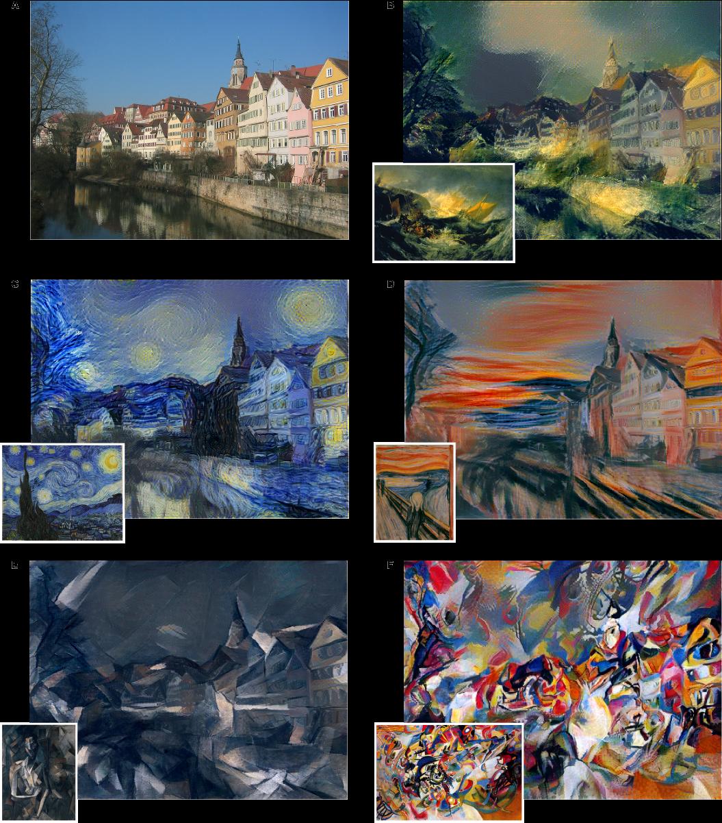
*One example input image with different styles added to it.*

-------------------------

### Rough chapter-wise notes

* Page 1
  * A painted image can be decomposed in its content and its artistic style.
  * Here they use a neural network to separate content and style from each other (and to apply that style to an existing image).

* Page 2
  * Representations get more abstract as you go deeper in networks, hence they should more resemble the actual content (as opposed to the artistic style).
  * They call the feature responses in higher layers *content representation*.
  * To capture style information, they use a method that was originally designed to capture texture information.
  * They somehow build a feature space on top of the existing one, that is somehow dependent on correlations of features. That leads to a "stationary" (?) and multi-scale representation of the style.

* Page 3
  * They use VGG as their base CNN.

* Page 4
  * Based on the extracted style features, they can generate a new image, which has equal activations in these style features.
  * The new image should match the style (texture, color, localized structures) of the artistic image.
  * The style features become more and more abtstract with higher layers. They call that multi-scale the *style representation*.
  * The key contribution of the paper is a method to separate style and content representation from each other.
  * These representations can then be used to change the style of an existing image (by changing it so that its content representation stays the same, but its style representation matches the artwork).

* Page 6
  * The generated images look most appealing if all features from the style representation are used. (The lower layers tend to reflect small features, the higher layers tend to reflect larger features.)
  * Content and style can't be separated perfectly.
  * Their loss function has two terms, one for content matching and one for style matching.
  * The terms can be increased/decreased to match content or style more.

* Page 8
  * Previous techniques work only on limited or simple domains or used non-parametric approaches (see non-photorealistic rendering).
  * Previously neural networks have been used to classify the time period of paintings (based on their style).
  * They argue that separating content from style might be useful and many other domains (other than transfering style of paintings to images).

* Page 9
  * The style representation is gathered by measuring correlations between activations of neurons.
  * They argue that this is somehow similar to what "complex cells" in the primary visual system (V1) do.
  * They note that deep convnets seem to automatically learn to separate content from style, probably because it is helpful for style-invariant classification.

* Page 9, Methods
  * They use the 19 layer VGG net as their basis.
  * They use only its convolutional layers, not the linear ones.
  * They use average pooling instead of max pooling, as that produced slightly better results.

* Page 10, Methods
  * The information about the image that is contained in layers can be visualized. To do that, extract the features of a layer as the labels, then start with a white noise image and change it via gradient descent until the generated features have minimal distance (MSE) to the extracted features.
  * The build a style representation by calculating Gram Matrices for each layer.

* Page 11, Methods
  * The Gram Matrix is generated in the following way:
    * Convert each filter of a convolutional layer to a 1-dimensional vector.
    * For a pair of filters i, j calculate the value in the Gram Matrix by calculating the scalar product of the two vectors of the filters.
    * Do that for every pair of filters, generating a matrix of size #filters x #filters. That is the Gram Matrix.
  * Again, a white noise image can be changed with gradient descent to match the style of a given image (i.e. minimize MSE between two Gram Matrices).
  * That can be extended to match the style of several layers by measuring the MSE of the Gram Matrices of each layer and giving each layer a weighting.

* Page 12, Methods
  * To transfer the style of a painting to an existing image, proceed as follows:
    * Start with a white noise image.
    * Optimize that image with gradient descent so that it minimizes both the content loss (relative to the image) and the style loss (relative to the painting).
    * Each distance (content, style) can be weighted to have more or less influence on the loss function.

A very simple (but impractical) discrete model of subclonal evolution would include the following events:

* Division of a cell to create two cells:
    * **Mutation** at a location in the genome of the new cells
* Cell death at a new timestep
* Cell survival at a new timestep

Because measurements of mutations are usually taken at one time point, this is taken to be at the end of a time series of these events, where a tiny of subset of cells are observed and a **genotype matrix** $A$ is produced, in which mutations and cells are arbitrarily indexed such that $A_{i,j} = 1$ if mutation $j$ exists in cell $i$. What this matrix allows us to see is the proportion of cells which *both have mutation $j$*.

Unfortunately, I don't get to observe $A$, in practice $A$ has been corrupted by IID binary noise to produce $A'$. This paper focuses on difference inference problems given $A'$, including *inferring $A$*, which is referred to as **`noise_elimination`**. The other problems involve inferring only properties of the matrix $A$, which are referred to as:

* **`noise_inference`**: predict whether matrix $A$ would satisfy the *three gametes rule*, which asks if a given genotype matrix *does not describe a branching phylogeny* because a cell has inherited mutations from two different cells (which is usually assumed to be impossible under the infinite sites assumption). This can be computed exactly from $A$.
* **Branching Inference**: it's possible that all mutations are inherited between the cells observed; in which case there are *no branching events*. The paper states that this can be computed by searching over permutations of the rows and columns of $A$. The problem is to predict from $A'$ if this is the case.

In both problems inferring properties of $A$, the authors use fully connected networks with two hidden layers on simulated datasets of matrices. For **`noise_elimination`**, computing $A$ given $A'$, the authors use a network developed for neural machine translation called a [pointer network][pointer]. They also find it necessary to map $A'$ to a matrix $A''$, turning every element in $A'$ to a fixed length row containing the location, mutation status and false positive/false negative rate.

Unfortunately, reported results on real datasets are reported only for branching inference and are limited by the restriction on input dimension. The inferred branching probability reportedly matches that reported in the literature.

[pointer]: https://arxiv.org/abs/1409.0473

Ongoing declines in production of the world's fisheries may have serious ecological and socioeconomic consequences. As a result, a number of international efforts have sought to improve management and prevent overexploitation, while helping to maintain biodiversity and a sustainable food supply. Although these initiatives have received broad acceptance, the extent to which corrective measures have been implemented and are effective remains largely unknown. We used a survey approach, validated with empirical data, and enquiries to over 13,000 fisheries experts (of which 1,188 responded) to assess the current effectiveness of fisheries management regimes worldwide; for each of those regimes, we also calculated the probable sustainability of reported catches to determine how management affects fisheries sustainability. Our survey shows that 7% of all coastal states undergo rigorous scientific assessment for the generation of management policies, 1.4% also have a participatory and transparent processes to convert scientific recommendations into policy, and 0.95% also provide for robust mechanisms to ensure the compliance with regulations; none is also free of the effects of excess fishing capacity, subsidies, or access to foreign fishing. A comparison of fisheries management attributes with the sustainability of reported fisheries catches indicated that the conversion of scientific advice into policy, through a participatory and transparent process, is at the core of achieving fisheries sustainability, regardless of other attributes of the fisheries. Our results illustrate the great vulnerability of the world's fisheries and the urgent need to meet well-identified guidelines for sustainable management; they also provide a baseline against which future changes can be quantified. Author Summary Top Global fisheries are in crisis: marine fisheries provide 15% of the animal protein consumed by humans, yet 80% of the world's fish stocks are either fully exploited, overexploited or have collapsed. Several international initiatives have sought to improve the management of marine fisheries, hoping to reduce the deleterious ecological and socioeconomic consequence of the crisis. Unfortunately, the extent to which countries are improving their management and whether such intervention ensures the sustainability of the fisheries remain unknown. Here, we surveyed 1,188 fisheries experts from every coastal country in the world for information about the effectiveness with which fisheries are being managed, and related those results to an index of the probable sustainability of reported catches. We show that the management of fisheries worldwide is lagging far behind international guidelines recommended to minimize the effects of overexploitation. Only a handful of countries have a robust scientific basis for management recommendations, and transparent and participatory processes to convert those recommendations into policy while also ensuring compliance with regulations. Our study also shows that the conversion of scientific advice into policy, through a participatory and transparent process, is at the core of achieving fisheries sustainability, regardless of other attributes of the fisheries. These results illustrate the benefits of participatory, transparent, and science-based management while highlighting the great vulnerability of the world's fisheries services. The data for each country can be viewed at http://as01.ucis.dal.ca/ramweb/surveys/fishery_assessment .