
|
Welcome to ShortScience.org! |


|
- ShortScience.org is a platform for post-publication discussion aiming to improve accessibility and reproducibility of research ideas.
- The website has 1584 public summaries, mostly in machine learning, written by the community and organized by paper, conference, and year.
- Reading summaries of papers is useful to obtain the perspective and insight of another reader, why they liked or disliked it, and their attempt to demystify complicated sections.
- Also, writing summaries is a good exercise to understand the content of a paper because you are forced to challenge your assumptions when explaining it.
- Finally, you can keep up to date with the flood of research by reading the latest summaries on our Twitter and Facebook pages.
Deep Networks with Stochastic Depth
Huang, Gao and Sun, Yu and Liu, Zhuang and Sedra, Daniel and Weinberger, Kilian
arXiv e-Print archive - 2016 via Local Bibsonomy
Keywords: deeplearning, acreuser
Huang, Gao and Sun, Yu and Liu, Zhuang and Sedra, Daniel and Weinberger, Kilian
arXiv e-Print archive - 2016 via Local Bibsonomy
Keywords: deeplearning, acreuser


[link]
**Dropout for layers** sums it up pretty well. The authors built on the idea of [deep residual networks](http://arxiv.org/abs/1512.03385) to use identity functions to skip layers. The main advantages: * Training speed-ups by about 25% * Huge networks without overfitting ## Evaluation * [CIFAR-10](https://www.cs.toronto.edu/~kriz/cifar.html): 4.91% error ([SotA](https://martin-thoma.com/sota/#image-classification): 2.72 %) Training Time: ~15h * [CIFAR-100](https://www.cs.toronto.edu/~kriz/cifar.html): 24.58% ([SotA](https://martin-thoma.com/sota/#image-classification): 17.18 %) Training time: < 16h * [SVHN](http://ufldl.stanford.edu/housenumbers/): 1.75% ([SotA](https://martin-thoma.com/sota/#image-classification): 1.59 %) - trained for 50 epochs, begging with a LR of 0.1, divided by 10 after 30 epochs and 35. Training time: < 26h  |

Adversarial Examples Are Not Bugs, They Are Features
Ilyas, Andrew and Santurkar, Shibani and Tsipras, Dimitris and Engstrom, Logan and Tran, Brandon and Madry, Aleksander
- 2019 via Local Bibsonomy
Keywords: adversarial
Ilyas, Andrew and Santurkar, Shibani and Tsipras, Dimitris and Engstrom, Logan and Tran, Brandon and Madry, Aleksander
- 2019 via Local Bibsonomy
Keywords: adversarial
|
[link]
Ilyas et al. present a follow-up work to their paper on the trade-off between accuracy and robustness. Specifically, given a feature $f(x)$ computed from input $x$, the feature is considered predictive if

$\mathbb{E}_{(x,y) \sim \mathcal{D}}[y f(x)] \geq \rho$;

similarly, a predictive feature is robust if

$\mathbb{E}_{(x,y) \sim \mathcal{D}}\left[\inf_{\delta \in \Delta(x)} yf(x + \delta)\right] \geq \gamma$.

This means, a feature is considered robust if the worst-case correlation with the label exceeds some threshold $\gamma$; here the worst-case is considered within a pre-defined set of allowed perturbations $\Delta(x)$ relative to the input $x$. Obviously, there also exist predictive features, which are however not robust according to the above definition. In the paper, Ilyas et al. present two simple algorithms for obtaining adapted datasets which contain only robust or only non-robust features. The main idea of these algorithms is that an adversarially trained model only utilizes robust features, while a standard model utilizes both robust and non-robust features. Based on these datasets, they show that non-robust, predictive features are sufficient to obtain high accuracy; similarly training a normal model on a robust dataset also leads to reasonable accuracy but also increases robustness. Experiments were done on Cifar10. These observations are supported by a theoretical toy dataset consisting of two overlapping Gaussians; I refer to the paper for details.

Also find this summary at [davidstutz.de](https://davidstutz.de/category/reading/).
|

InfoGAN: Interpretable Representation Learning by Information Maximizing Generative Adversarial Nets
Chen, Xi and Chen, Xi and Duan, Yan and Houthooft, Rein and Schulman, John and Sutskever, Ilya and Abbeel, Pieter
Neural Information Processing Systems Conference - 2016 via Local Bibsonomy
Keywords: dblp
Chen, Xi and Chen, Xi and Duan, Yan and Houthooft, Rein and Schulman, John and Sutskever, Ilya and Abbeel, Pieter
Neural Information Processing Systems Conference - 2016 via Local Bibsonomy
Keywords: dblp
|
[link]
* Usually GANs transform a noise vector `z` into images. `z` might be sampled from a normal or uniform distribution.
* The effect of this is, that the components in `z` are deeply entangled.
* Changing single components has hardly any influence on the generated images. One has to change multiple components to affect the image.
* The components end up not being interpretable. Ideally one would like to have meaningful components, e.g. for human faces one that controls the hair length and a categorical one that controls the eye color.
* They suggest a change to GANs based on Mutual Information, which leads to interpretable components.
* E.g. for MNIST a component that controls the stroke thickness and a categorical component that controls the digit identity (1, 2, 3, ...).
* These components are learned in a (mostly) unsupervised fashion.
### How
* The latent code `c`
* "Normal" GANs parameterize the generator as `G(z)`, i.e. G receives a noise vector and transforms it into an image.
* This is changed to `G(z, c)`, i.e. G now receives a noise vector `z` and a latent code `c` and transforms both into an image.
* `c` can contain multiple variables following different distributions, e.g. in MNIST a categorical variable for the digit identity and a gaussian one for the stroke thickness.
* Mutual Information
* If using a latent code via `G(z, c)`, nothing forces the generator to actually use `c`. It can easily ignore it and just deteriorate to `G(z)`.
* To prevent that, they force G to generate images `x` in a way that `c` must be recoverable. So, if you have an image `x` you must be able to reliable tell which latent code `c` it has, which means that G must use `c` in a meaningful way.
* This relationship can be expressed with mutual information, i.e. the mutual information between `x` and `c` must be high.
* The mutual information between two variables X and Y is defined as `I(X; Y) = entropy(X) - entropy(X|Y) = entropy(Y) - entropy(Y|X)`.
* If the mutual information between X and Y is high, then knowing Y helps you to decently predict the value of X (and the other way round).
* If the mutual information between X and Y is low, then knowing Y doesn't tell you much about the value of X (and the other way round).
* The new GAN loss becomes `old loss - lambda * I(G(z, c); c)`, i.e. the higher the mutual information, the lower the result of the loss function.
* Variational Mutual Information Maximization
* In order to minimize `I(G(z, c); c)`, one has to know the distribution `P(c|x)` (from image to latent code), which however is unknown.
* So instead they create `Q(c|x)`, which is an approximation of `P(c|x)`.
* `I(G(z, c); c)` is then computed using a lower bound maximization, similar to the one in variational autoencoders (called "Variational Information Maximization", hence the name "InfoGAN").
* Basic equation: `LowerBoundOfMutualInformation(G, Q) = E[log Q(c|x)] + H(c) <= I(G(z, c); c)`
* `c` is the latent code.
* `x` is the generated image.
* `H(c)` is the entropy of the latent codes (constant throughout the optimization).
* Optimization w.r.t. Q is done directly.
* Optimization w.r.t. G is done via the reparameterization trick.
* If `Q(c|x)` approximates `P(c|x)` *perfectly*, the lower bound becomes the mutual information ("the lower bound becomes tight").
* In practice, `Q(c|x)` is implemented as a neural network. Both Q and D have to process the generated images, which means that they can share many convolutional layers, significantly reducing the extra cost of training Q.
### Results
* MNIST
* They use for `c` one categorical variable (10 values) and two continuous ones (uniform between -1 and +1).
* InfoGAN learns to associate the categorical one with the digit identity and the continuous ones with rotation and width.
* Applying Q(c|x) to an image and then classifying only on the categorical variable (i.e. fully unsupervised) yields 95% accuracy.
* Sampling new images with exaggerated continuous variables in the range `[-2,+2]` yields sound images (i.e. the network generalizes well).
* 
* 3D face images
* InfoGAN learns to represent the faces via pose, elevation, lighting.
* They used five uniform variables for `c`. (So two of them apparently weren't associated with anything sensible? They are not mentioned.)
* 3D chair images
* InfoGAN learns to represent the chairs via identity (categorical) and rotation or width (apparently they did two experiments).
* They used one categorical variable (four values) and one continuous variable (uniform `[-1, +1]`).
* SVHN
* InfoGAN learns to represent lighting and to spot the center digit.
* They used four categorical variables (10 values each) and two continuous variables (uniform `[-1, +1]`). (Again, a few variables were apparently not associated with anything sensible?)
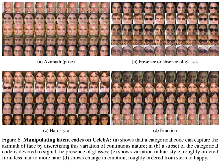
* CelebA
* InfoGAN learns to represent pose, presence of sunglasses (not perfectly), hair style and emotion (in the sense of "smiling or not smiling").
* They used 10 categorical variables (10 values each). (Again, a few variables were apparently not associated with anything sensible?)
* 
|

Inception-v4, Inception-ResNet and the Impact of Residual Connections on Learning
Szegedy, Christian and Ioffe, Sergey and Vanhoucke, Vincent
arXiv e-Print archive - 2016 via Local Bibsonomy
Keywords: dblp
Szegedy, Christian and Ioffe, Sergey and Vanhoucke, Vincent
arXiv e-Print archive - 2016 via Local Bibsonomy
Keywords: dblp
|
[link]
This paper presents a combination of the inception architecture with residual networks. This is done by adding a shortcut connection to each inception module. This can alternatively be seen as a resnet where the 2 conv layers are replaced by a (slightly modified) inception module. The paper (claims to) provide results against the hypothesis that adding residual connections improves training, rather increasing the model size is what makes the difference. |

Value Prediction Network
Oh, Junhyuk and Singh, Satinder and Lee, Honglak
arXiv e-Print archive - 2017 via Local Bibsonomy
Keywords: dblp
Oh, Junhyuk and Singh, Satinder and Lee, Honglak
arXiv e-Print archive - 2017 via Local Bibsonomy
Keywords: dblp
|
[link]
Recently, DeepMind released a new paper showing strong performance on board game tasks using a mechanism similar to the Value Prediction Network one in this paper, which inspired me to go back and get a grounding in this earlier work. A goal of this paper is to design a model-based RL approach that can scale to complex environment spaces, but can still be used to run simulations and do explicit planning. Traditional, model-based RL has worked by learning a dynamics model of the environment - predicting the next observation state given the current one and an action, and then using that model of the world to learn values and plan with. In addition to the advantages of explicit planning, a hope is that model-based systems generalize better to new environments, because they predict one-step changes in local dynamics in a way that can be more easily separated from long-term dynamics or reward patterns. However, a downside of MBRL is that it can be hard to train, especially when your observation space is high-dimensional, and learning a straight model of your environment will lead to you learning details that aren't actually unimportant for planning or creating policies. The synthesis proposed by this paper is the Value Prediction Network. Rather than predicting observed state at the next step, it learns a transition model in latent space, and then learns to predict next-step reward and future value from that latent space vector. Because it learns to encode latent-space state from observations, and also learns a transition model from one latent state to another, the model can be used for planning, by simulating multiple transitions between latent state. However, unlike a normal dynamics model, whose training signal comes from a loss against observational prediction, the signal for training both latent → reward/value/discount predictions, and latent → latent transitions comes from using this pipeline to predict reward values. This means that if an aspect of the environment isn't useful for predicting reward, it won't generally be encoded into latent state, meaning you don't waste model capacity predicting irrelevant detail. https://i.imgur.com/4bJylms.png Once this model exists, it can be used for generating a policy through a tree-search planning approach: simulating future trajectories and aggregating the predicted reward along those trajectories, and then taking the highest-value one. The authors find that their model is able to do better than both model-free and model-based methods on the tasks they tested on. In particular, they find that it has many of the benefits of a model that predicts full observations, but that the Value Prediction Network learns more quickly, and is more robust to stochastic environments where there's an inherent ceiling on how well a next-step observation prediction can work. My main question coming into this paper is: how is this different from simply a value estimator like those used in DQN or A2C, and my impression is that the difference comes from this model's ability to do explicit state simulation in latent space, and then predict a value off of the *latent* state, whereas a value network predicts value from observational state. |
