The paper provides derivations and intuitions about the learning dynamics for VAEs based on observations about [$\beta$-VAEs][beta]. Using this they derive an alternative way to constrain the training of VAEs that doesn't require typical heuristics, such as warmup or adding noise to the data.

How exactly would this change a typical implementation? Typically, SGD is used to [optimize the ELBO directly](https://github.com/pytorch/examples/blob/master/vae/main.py#L91-L95). Using GECO, I keep a moving average of my constraint $C$ (chosen based on what I want the VAE to do, but it can be just the likelihood plus a tolerance parameter) and use that to calculate Lagrange multipliers, which control the weighting of the constraint to the loss. [This implementation](https://github.com/denproc/Taming-VAEs/blob/master/train.py#L83-L97) from a class project appears to be correct.

With the stabilization of training, I can't help but think of this as batchnorm for VAEs.

[beta]: https://openreview.net/forum?id=Sy2fzU9gl

[Hive](http://infolab.stanford.edu/~ragho/hive-icde2010.pdf) is an open-source data warehousing solution built on top of Hadoop.  It supports an SQL-like query language called HiveQL. These queries are compiled into MapReduce jobs that are executed on Hadoop. While Hive uses Hadoop for execution of queries, it reduces the effort that goes into writing and maintaining MapReduce jobs.

# Data Model

Hive supports database concepts like tables, columns, rows and partitions. Both primitive (integer, float, string) and complex data-types(map, list, struct) are supported. Moreover, these types can be composed to support structures of arbitrary complexity. The tables are serialized/deserialized using default serializers/deserializer. Any new data format and type can be supported by implementing SerDe and ObjectInspector java interface.

# Query Language

Hive query language (HiveQL) consists of a subset of SQL along with some extensions. The language is very SQL-like and supports features like subqueries, joins, cartesian product, group by, aggregation, describe and more. MapReduce programs can also be used in Hive queries. A sample query using MapReduce would look like this:

```
FROM ( 
    MAP inputdata USING 'python mapper.py' AS (word, count)
    FROM inputtable
    CLUSTER BY word
    )
    REDUCE word, count USING 'python reduce.py';
```
This query uses `mapper.py` for transforming `inputdata` into `(word, count)` pair, distributes data to reducers by hashing on `word` column (given by `CLUSTER`) and uses `reduce.py`.

Notice that Hive allows the order of `FROM` and `SELECT/MAP/REDUCE` to be changed within a sub-query. This allows insertion of different transformation results into different tables/partitions/hdfs/local directory as part of the same query and reduces the number of scans on the input data.

### Limitations

* Only equi-joins are supported.
* Data can not be inserted into existing table/partitions and all inserts overwrite the data. 

`INSERT INTO, UPDATE`, and `DELETE` are not supported which makes it easier to handle reader and writer concurrency.

# Data Storage

While a table is the logical data unit in Hive, the data is actually stored into hdfs directories. A **table** is stored as a directory in hdfs, **partition** of a table as a subdirectory within a directory and **bucket** as a file within the table/partition directory. Partitions can be created either when creating tables or by using `INSERT/ALTER` statement. The partitioning information is used to prune data when running queries. For example, suppose we create partition for `day=monday` using the query

```
ALTER TABLE dummytable ADD PARTITION (day='monday')
```
Next, we run the query - 
```
SELECT * FROM dummytable WHERE day='monday'
```
Suppose the data in dummytable is stored in `/user/hive/data/dummytable` directory. This query will only scan the subdirectory `/user/hive/data/dummytable/day=monday` within the `dummytable` directory.

A **bucket** is a file within the leaf directory of a table or a partition. It can be used to prune data when the user runs a `SAMPLE` query. 

Any data stored in hdfs can be queried using the `EXTERNAL TABLE` clause by specifying its location with the `LOCATION` clause. When dropping an external table, only its metadata is deleted and not the data itself.

# Serialization/Deserialization

Hive implements the `LazySerDe` as the default SerDe. It deserializes rows into internal objects lazily so that the cost of Deserialization of a column is incurred only when it is needed. Hive also provides a `RegexSerDe` which allows the use of regular expressions to parse columns out from a row. Hive also supports various formats like `TextInputFormat`, `SequenceFileInputFormat` and `RCFileInputFormat`. Other formats can also be implemented and specified in the query itself. For example, 

```
CREATE TABLE dummytable(key INT, value STRING)
    STORED AS 
        INPUTFORMAT
            org.apache.hadoop.mapred.SequenceFileInputFormat
        OUTPUTFORMAT
            org.apache.hadoop.mapred.SequenceFileOutputFormat
```

# System Architecture and Component

### Components

* **Metastore** - Stores system catalog and metadata about tables, columns and partitions.
* **Driver** - Manages life cycle of a HiveQL statement as it moves through Hive.
* **Query Compiler** - Compiles query into a directed acyclic graph of MapReduce tasks.
* **Execution Engine** - Execute tasks produced by the compiler in proper dependency order.
* **Hive Server** - Provides a thrift interface and a JDBC/ODBC server.
* **Client components** - CLI, web UI, and JDBC/ODBC driver.
* **Extensibility Interfaces** - Interfaces for SerDe, ObjectInspector, UDF (User Defined Function) and UDAF (User-Defined Aggregate Function).

### Life Cycle of a query

The query is submitted via CLI/web UI/any other interface. This query goes to the compiler and undergoes parse, type-check and semantic analysis phases using the metadata from Metastore. The compiler generates a logical plan which is optimized by the rule-based optimizer and an optimized plan in the form of DAG of MapReduce and hdfs tasks is generated. The execution engine executes these tasks in the correct order using Hadoop.

### Metastore
It stores all information about the tables, their partitions, schemas, columns and their types, etc. Metastore runs on traditional RDBMS (so that latency for metadata query is very small) and uses an open source ORM layer called DataNuclues. Matastore is backed up regularly. To make sure that the system scales with the number of queries, no metadata queries are made the mapper/reducer of a job. Any metadata needed by the mapper or the reducer is passed through XML plan files that are generated by the compiler.

### Query Compiler

Hive Query Compiler works similar to traditional database compilers.
* Antlr is used to generate the Abstract Syntax Tree (AST) of the query.
* A logical plan is created using information from the metastore. An intermediate representation called query block (QB) tree is used when transforming AST to operator DAG. Nested queries define the parent-child relationship in QB tree.
* Optimization logic consists of a chain of transformation operations such that output from one operation is input to next operation. Each transformation comprises of a **walk** on operator DAG. Each visited **node** in the DAG is tested for different **rules**. If any rule is satisfied, its corresponding **processor** is invoked. **Dispatcher** maintains a mapping fo different rules and their processors and does rule matching. **GraphWalker** manages the overall traversal process.
* Logical plan generated in the previous step is split into multiple MapReduce and hdfs tasks. Nodes in the plan correspond to physical operators and edges represent the flow of data between operators.

### Optimisations     

* **Column Pruning** - Only the columns needed in the query processing are projected.
* **Predicate Pushdown** - Predicates are pushed down to the scan so that rows are filtered as early as possible.
* **Partition Pruning** - Predicates on partitioned columns are used to prune out files of partitions that do not satisfy the predicate. 
* **Map Side Joins** - In case the tables involved in the join are very small, the tables are replicated in all the mappers and the reducers.
* **Join Reordering** - Large tables are streamed and not materialized in-memory in the reducer to reduce memory requirements.

Some optimizations are not enabled by default but can be activated by setting certain flags. These include: 

* Repartitioning data to handle skew in `GROUP BY` processing.This is achieved by performing `GROUP BY` in two MapReduce stages - first where data is distributed randomly to the reducers and partial aggregation is performed. In the second stage, these partial aggregations are distributed on GROUP BY columns to different reducers.
* Hash bases partial aggregations in the mappers to reduce the data that is sent by the mappers to the reducers which help in reducing the amount of time spent in sorting and merging the resulting data.

### Execution Engine

Execution Engine executes the tasks in order of their dependencies. A MapReduce task first serializes its part of the plan into a plan.xml file. This file is then added to the job cache and mappers and reducers are spawned to execute relevant sections of the operator DAG. The final results are stored to a temporary location and then moved to the final destination (in the case of say `INSERT INTO` query).

# Future Work

The paper mentions the following areas for improvements:

* HiveQL should subsume SQL syntax.
* Implementing a cost-based optimizer and using adaptive optimization techniques.
* Columnar storage to improve scan performance.
* Enhancing JDBS/ODBC drivers for Hive to integrate with other BI tools.
* Multi-query optimization and generic n-way join in a single MapReduce job.

  * DRAW = deep recurrent attentive writer
  * DRAW is a recurrent autoencoder for (primarily) images that uses attention mechanisms.
  * Like all autoencoders it has an encoder, a latent layer `Z` in the "middle" and a decoder.
  * Due to the recurrence, there are actually multiple autoencoders, one for each timestep (the number of timesteps is fixed).
  * DRAW has attention mechanisms which allow the model to decide where to look at in the input image ("glimpses") and where to write/draw to in the output image.
  * If the attention mechanisms are skipped, the model becomes a simple recurrent autoencoder.
  * By training the full autoencoder on a dataset and then only using the decoder, one can generate new images that look similar to the dataset images.


![DRAW Architecture](https://raw.githubusercontent.com/aleju/papers/master/neural-nets/images/DRAW_A_Recurrent_Neural_Network_for_Image_Generation__architecture.png?raw=true "DRAW Architecture")

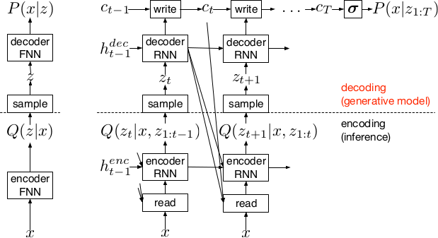
*Basic recurrent architecture of DRAW.*


### How
  * General architecture
    * The encoder-decoder-pair follows the design of variational autoencoders.
    * The latent layer follows an n-dimensional gaussian distribution. The hyperparameters of that distribution (means, standard deviations) are derived from the output of the encoder using a linear transformation.
    * Using a gaussian distribution enables the use of the reparameterization trick, which can be useful for backpropagation.
    * The decoder receives a sample drawn from that gaussian distribution.
    * While the encoder reads from the input image, the decoder writes to an image canvas (where "write" is an addition, not a replacement of the old values).
    * The model works in a fixed number of timesteps. At each timestep the encoder performs a read operation and the decoder a write operation.
    * Both the encoder and the decoder receive the previous output of the encoder.
  * Loss functions
    * The loss function of the latent layer is the KL-divergence between that layer's gaussian distribution and a prior, summed over the timesteps.
    * The loss function of the decoder is the negative log likelihood of the image given the final canvas content under a bernoulli distribution.
    * The total loss, which is optimized, is the expectation of the sum of both losses (latent layer loss, decoder loss).
  * Attention
    * The selective read attention works on image patches of varying sizes. The result size is always NxN.
    * The mechanism has the following parameters:
        * `gx`: x-axis coordinate of the center of the patch
        * `gy`: y-axis coordinate of the center of the patch
        * `delta`: Strides. The higher the strides value, the larger the read image patch.
        * `sigma`: Standard deviation. The higher the sigma value, the more blurry the extracted patch will be.
        * `gamma`: Intensity-Multiplier. Will be used on the result.
        * All of these parameters are generated using a linear transformation applied to the decoder's output.
    * The mechanism places a grid of NxN gaussians on the image. The grid is centered at `(gx, gy)`. The gaussians are `delta` pixels apart from each other and have a standard deviation of `sigma`.
    * Each gaussian is applied to the image, the center pixel is read and added to the result.


![DRAW Attention](https://raw.githubusercontent.com/aleju/papers/master/neural-nets/images/DRAW_A_Recurrent_Neural_Network_for_Image_Generation__attention.png?raw=true "DRAW Attention")

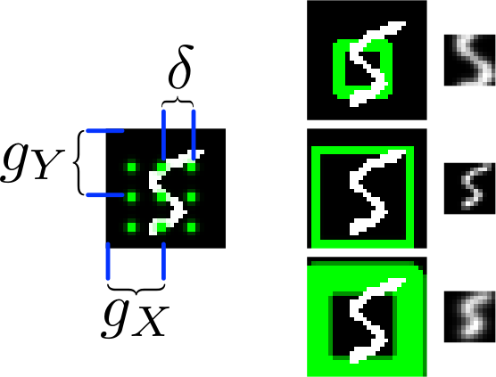
*The basic attention mechanism. (gx, gy) is the read patch center. delta is the strides. On the right: Patches with different sizes/strides and standard deviations/blurriness.*


### Results
  * Realistic looking generated images for MNIST and SVHN.
  * Structurally OK, but overall blurry images for CIFAR-10.
  * Results with attention are usually significantly better than without attention.
  * Image generation without attention starts with a blurry image and progressively sharpens it.

![DRAW SVHN Results](https://raw.githubusercontent.com/aleju/papers/master/neural-nets/images/DRAW_A_Recurrent_Neural_Network_for_Image_Generation__svhn.png?raw=true "DRAW SVHN Results")

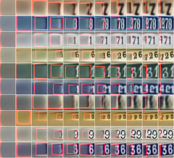
*Using DRAW with attention to generate new SVHN images.*

----------

### Rough chapter-wise notes

* 1. Introduction
  * The natural way to draw an image is in a step by step way (add some lines, then add some more, etc.).
  * Most generative neural networks however create the image in one step.
  * That removes the possibility of iterative self-correction, is hard to scale to large images and makes the image generation process dependent on a single latent distribution (input parameters).
  * The DRAW architecture generates images in multiple steps, allowing refinements/corrections.
  * DRAW is based on varational autoencoders: An encoder compresses images to codes and a decoder generates images from codes.
  * The loss function is a variational upper bound on the log-likelihood of the data.
  * DRAW uses recurrance to generate images step by step.
  * The recurrance is combined with attention via partial glimpses/foveations (i.e. the model sees only a small part of the image).
  * Attention is implemented in a differentiable way in DRAW.

* 2. The DRAW Network
  * The DRAW architecture is based on variational autoencoders:
    * Encoder: Compresses an image to latent codes, which represent the information contained in the image.
    * Decoder: Transforms the codes from the encoder to images (i.e. defines a distribution over images which is conditioned on the distribution of codes).
  * Differences to variational autoencoders:
    * Encoder and decoder are both recurrent neural networks.
    * The encoder receives the previous output of the decoder.
    * The decoder writes several times to the image array (instead of only once).
    * The encoder has an attention mechanism. It can make a decision about the read location in the input image.
    * The decoder has an attention mechanism. It can make a decision about the write location in the output image.
  * 2.1 Network architecture
    * They use LSTMs for the encoder and decoder.
    * The encoder generates a vector.
    * The decoder generates a vector.
    * The encoder receives at each time step the image and the output of the previous decoding step.
    * The hidden layer in between encoder and decoder is a distribution Q(Zt|ht^enc), which is a diagonal gaussian.
    * The mean and standard deviation of that gaussian is derived from the encoder's output vector with a linear transformation.
    * Using a gaussian instead of a bernoulli distribution enables the use of the reparameterization trick. That trick makes it straightforward to backpropagate "low variance stochastic gradients of the loss function through the latent distribution".
    * The decoder writes to an image canvas. At every timestep the vector generated by the decoder is added to that canvas.
  * 2.2 Loss function
    * The main loss function is the negative log probability: `-log D(x|ct)`, where `x` is the input image and `ct` is the final output image of the autoencoder. `D` is a bernoulli distribution if the image is binary (only 0s and 1s).
    * The model also uses a latent loss for the latent layer (between encoder and decoder). That is typical for VAEs. The loss is the KL-Divergence between Q(Zt|ht_enc) (`Zt` = latent layer, `ht_enc` = result of encoder) and a prior `P(Zt)`.
    * The full loss function is the expection value of both losses added up.
  * 2.3 Stochastic Data Generation
    * To generate images, samples can be picked from the latent layer based on a prior. These samples are then fed into the decoder. That is repeated for several timesteps until the image is finished.

* 3. Read and Write Operations
  * 3.1 Reading and writing without attention
    * Without attention, DRAW simply reads in the whole image and modifies the whole output image canvas at every timestep.
  * 3.2 Selective attention model
    * The model can decide which parts of the image to read, i.e. where to look at. These looks are called glimpses.
    * Each glimpse is defined by its center (x, y), its stride (zoom level), its gaussian variance (the higher the variance, the more blurry is the result) and a scalar multiplier (that scales the intensity of the glimpse result).
    * These parameters are calculated based on the decoder output using a linear transformation.
    * For an NxN patch/glimpse `N*N` gaussians are created and applied to the image. The center pixel of each gaussian is then used as the respective output pixel of the glimpse.
  * 3.3 Reading and writing with attention
    * Mostly the same technique from (3.2) is applied to both reading and writing.
    * The glimpse parameters are generated from the decoder output in both cases. The parameters can be different (i.e. read and write at different positions).
    * For RGB the same glimpses are applied to each channel.

* 4. Experimental results
  * They train on binary MNIST, cluttered MNIST, SVHN and CIFAR-10.
  * They then classfiy the images (cluttered MNIST) or generate new images (other datasets).
  * They say that these generated images are unique (to which degree?) and that they look realistic for MNIST and SVHN.
  * Results on CIFAR-10 are blurry.
  * They use binary crossentropy as the loss function for binary MNIST.
  * They use crossentropy as the loss function for SVHN and CIFAR-10 (color).
  * They used Adam as their optimizer.
  * 4.1 Cluttered MNIST classification
    * They classify images of cluttered MNIST. To do that, they use an LSTM that performs N read-glimpses and then classifies via a softmax layer.
    * Their model's error rate is significantly below a previous non-differentiable attention based model.
    * Performing more glimpses seems to decrease the error rate further.
  * 4.2 MNIST generation
    * They generate binary MNIST images using only the decoder.
    * DRAW without attention seems to perform similarly to previous models.
    * DRAW with attention seems to perform significantly better than previous models.
    * DRAW without attention progressively sharpens images.
    * DRAW with attention draws lines by tracing them.
  * 4.3 MNIST generation with two digits
    * They created a dataset of 60x60 images, each of them containing two random 28x28 MNIST images.
    * They then generated new images using only the decoder.
    * DRAW learned to do that.
    * Using attention, the model usually first drew one digit then the other.
  * 4.4 Street view house number generation
    * They generate SVHN images using only the decoder.
    * Results look quite realistic.
  * 4.5 Generating CIFAR images
    * They generate CIFAR-10 images using only the decoder.
    * Results follow roughly the structure of CIFAR-images, but look blurry.

Motivated by JPEG compression, Prakash et al. propose an adaptive quantization scheme as defense against adversarial attacks. They argue that JPEG experimentally reduces adversarial noise; however, it is difficult to automatically decide on the level of compression as it also influences a classifier’s performance. Therefore, Prakash et al. use a saliency detector to identify background region, and then apply adaptive quantization – with coarser detail at the background – to reduce the impact of adversarial noise. In experiments, they demonstrate that this approach outperforms simple  JPEG compression as defense while having less impact on the image quality.

Also find this summary at [davidstutz.de](https://davidstutz.de/category/reading/).

Current work in image generation (and generative models more broadly) can be split into two broad categories: implicit models, and likelihood-based models. Implicit models is a categorically that predominantly creates GANs, and which learns how to put pixels in the right places without actually learning a joint probability model over pixels. This is a detriment for applications where you do actually want to be able to calculate probabilities for particular images, in addition to simply sampling new images from your model. Within the class of explicit probability models, the auto-encoder and the autoregressive model are the two most central and well-established. 

An auto-encoder works by compressing information about an image into a central lower-dimensional “bottleneck” code, and then trying to reconstruct the original image using the information contained in the code. This structure works well for capturing global structure, but is generally weaker at local structure, because by convention images are generated through stacked convolutional layers, where each pixel in the image is sampled separately, albeit conditioned on the same latent state (the value of the layer below). This is in contrast to an auto-regressive decoder, where you apply some ordering to the pixels, and then sample them in sequence: starting the prior over the first pixel, and then the second conditional on the first, and so on. In this setup, instead of simply expecting your neighboring pixels to coordinate with you because you share latent state, the model actually has visibility into the particular pixel sampled at the prior step, and has the ability to condition on that. This leads to higher-precision generation of local pixel structure with these models .

If you want a model that can get the best of all of these worlds - high-local precision, good global structure, and the ability to calculate probabilities - a sensible approach might be to combine the two: to learn a global-compressed code using an autoencoder, and then, conditioning on that autoencoder code as well as the last sampled values, generate pixels using an autoregressive decoder. However, in practice, this has proved tricky. At a high level, this is because the two systems are hard to balance with one another, and different kinds of imbalance lead to different failure modes. If you try to constrain the expression power of your global code too much, your model will just give up on having global information, and just condition pixels on surrounding (past-sampled) pixels. But, by contrast, if you don’t limit the capacity of the code, then the model puts even very local information into the code and ignores the autoregressive part of the model, which brings it away from playing our desired role as global specifier of content. 

This paper suggests a new combination approach, whereby we jointly train an encoder and autoregressive decoder, but instead of training the encoder on the training signal produced by that decoder, we train it on the training signal we would have gotten from decoding the code into pixels using a simpler decoder, like a feedforward network. The autoregressive network trains on the codes from the encoder as the encoder trains, but it doesn’t actually pass any signal back to it. Basically, we’re training our global code to believe it’s working with a less competent decoder, and then substituting our autoregressive decoder in during testing. 

https://i.imgur.com/d2vF2IQ.png

Some additional technical notes: 
- Instead of using a more traditional continuous-valued bottleneck code, this paper uses the VQ-VAE tactic of discretizing code values, to be able to more easily control code capacity. This essentially amounts to generating code vectors as normal, clustering them, passing their cluster medians forward, and then ignoring the fact that none of this is differentiable and passing back gradients with respect to the median 
- For their auxiliary decoders, the authors use both a simple feedforward network, and also a more complicated network, where the model needs to guess a pixel, using only the pixel values outside of a window of size of that pixel. The goal of the latter variant is to experiment with a decoder that can’t use local information, and could only use global