
arXiv is an e-print service in the fields of physics, mathematics, computer science, quantitative biology, quantitative finance and statistics.
- 1996 1
- 2010 1
- 2011 1
- 2012 8
- 2013 31
- 2014 43
- 2015 134
- 2016 231
- 2017 182
- 2018 141
- 2019 100
- 2020 33
- 2021 10
- 2022 7
- 2023 3
Automatic chemical design using a data-driven continuous representation of molecules
Gómez-Bombarelli, Rafael and Duvenaud, David and Hernández-Lobato, José Miguel and Aguilera-Iparraguirre, Jorge and Hirzel, Timothy D. and Adams, Ryan P. and Aspuru-Guzik, Alán
arXiv e-Print archive - 2016 via Local Bibsonomy
Keywords: dblp
Gómez-Bombarelli, Rafael and Duvenaud, David and Hernández-Lobato, José Miguel and Aguilera-Iparraguirre, Jorge and Hirzel, Timothy D. and Adams, Ryan P. and Aspuru-Guzik, Alán
arXiv e-Print archive - 2016 via Local Bibsonomy
Keywords: dblp


[link]
I'll admit that I found this paper a bit of a letdown to read, relative to expectations rooted in its high citation count, and my general excitement and interest to see how deep learning could be brought to bear on molecular design. But before a critique, let's first walk through the mechanics of how the authors' approach works. The method proposed is basically a very straightforward Variational Auto Encoder, or VAE. It takes in a textual SMILES string representation of a molecular structure, uses an encoder to map that into a continuous vector representation, a decoder to map the vector representation back into a a SMILES string, and an auxiliary predictor to predict properties of a molecule given the continuous representation. So, the training loss is a combination of the reconstruction loss (log probability of the true molecule under the distribution produced by the decoder) and the semi-supervised predictive loss. The hope with this model is that it would allow you to sample from a space of potential molecules by starting from an existing molecule, and then optimizing the the vector representation of that molecule to make it score higher on whatever property you want to optimize for. https://i.imgur.com/WzZsCOB.png The authors acknowledge that, in this setup, you're just producing a probability distribution over characters, and that the continuous vectors sampled from the latent space might not actually map to valid SMILES strings, and beyond that may well not correspond to chemically valid molecules. Empirically, they said that the proportion of valid generated molecules ranged between 1 and 70%. But they argue that it'd be too difficult to enforce those constraints, and instead just sample from the model and run the results through a hand-designed filter for molecular validity. In my view, this is the central weakness of the method proposed in this paper: that they seem to have not tackled the question of either chemical viability or even syntactic correctness of the produced molecules. I found it difficult to nail down from the paper what the ultimate percentage of valid molecules was from points in latent space that were off of the training . A table reports "percentage of 5000 randomly-selected latent points that decode to valid molecules after 1000 attempts," but I'm confused by what the 1000 attempts means here - does that mean we draw 1000 samples from the distribution given by the decoder, and see if *any* of those samples are valid? That would be a strange metric, if so, and perhaps it means something different, but it's hard to tell. https://i.imgur.com/9sy0MXB.png This paper made me really curious to see whether a GAN could do better in this space, since it would presumably be better at the task of incentivizing syntactic correctness of produced strings (given that any deviation from correctness could be signal for the discriminator), but it might also lead to issues around mode collapse, and when I last checked the literature, GANs on text data in particular were still not great.  |

Low Data Drug Discovery with One-shot Learning
Altae-Tran, Han and Ramsundar, Bharath and Pappu, Aneesh S. and Pande, Vijay S.
arXiv e-Print archive - 2016 via Local Bibsonomy
Keywords: dblp
Altae-Tran, Han and Ramsundar, Bharath and Pappu, Aneesh S. and Pande, Vijay S.
arXiv e-Print archive - 2016 via Local Bibsonomy
Keywords: dblp
|
[link]
The goal of one-shot learning tasks is to design a learning structure that can perform a new task (or, more canonically, add a new class to an existing task) using only one a small number of examples of the new task or class. So, as an example: you'd want to be able to take one positive and one negative example of a given task and correctly classify subsequent points as either positive or negative. A common way of achieving this, and the way that the paper builds on, is to learn a parametrized function projecting both your labeled points (your "support set") and your unlabeled point (your "query") into an embedding space, and then assigning a class to your query according to how close it is to the support set points associated with each label. The hope is that, in the course of training on different but similar tasks, you've learned a metric space where nearby things tend to be of similar classes. This method is called a "matching network". This paper has the specific objective of using such one-shot methods for drug discovery, and evaluates on tasks drawn from that domain, but most of the mechanics of the paper can be understood without reference to molecular dat in particular. In the simplest version of such a network, the query and support set points are embedded unconditionally - meaning that the query would be embedded in the same way regardless of the values in the support set, and that each point in the support set would be embedded without knowledge of each other. However, given how little data we're giving our model to work with, it might be valuable to allow our query embedder (f(x)) and support set embedder (g(x)) to depend on the values within the support set. Prior work had achieved this by: 1) Creating initial f'(x) and g'(x) query and support embedders. 2) Concatenating the embedded support points g'(x) into a single vector and running a bidirectional LSTM over the concatenation, which results in a representation g(x) of each input that incorporates information from g'(x_i) for all other x_i (albeit in a way that imposes a concatenation ordering that may not correspond to a meaningful order) 3) Calculating f(x) of your embedding point by using an attention mechanism to combine f'(x) with the contextualized embeddings g(x) The authors of the current paper argue that this approach is suboptimal because of the artificially imposed ordering, and because it calculated g(x) prior to f(x) using asymmetrical model structures (though it's not super clear why this latter point is a problem). Instead, they propose a somewhat elaborate and difficult-to-follow attention based mechanism. As best as I can understand, this is what they're suggesting: https://i.imgur.com/4DLWh8H.png 1) Update the query embedding f(x) by calculating an attention distribution over the vector current embeddings of support set points (here referred to as bolded <r>), pooling downward to a single aggregate embedding vector r, and then using a LSTM that takes in that aggregate vector and the prior update to generate a new update. This update, dz, is added to the existing query embedding estimate to get a new one 2) Update the vector of support set embeddings by iteratively calculating an attention mapping between the vector of current support set embeddings and the original features g'(S), and using that attention mapping to create a new <r>, which, similar to the above, is fed into an LSTM to calculate the next update. Since the model is evaluated on molecular tasks, all of the embedding functions are structured as graph convolutions. Other than the obvious fact that attention is a great way of aggregating information in an order-independent way, the authors give disappointingly little justification of why they would expect their method to work meaningfully better than past approaches. Empirically, they do find that it performs slightly better than prior contextualized matching networks on held out tasks of predicting toxicity and side effects with only a small number from the held out task. However, neither this paper's new method nor previous one-shot learning work is able to perform very well on the challenging MUV dataset, where held-out binding tasks involve structurally dissimilar molecules from those seen during training, suggesting that whatever generalization this method is able to achieve doesn't quite rise to the task of making inferences based on molecules with different structures. |
Molecular Graph Convolutions: Moving Beyond Fingerprints
Kearnes, Steven M. and McCloskey, Kevin and Berndl, Marc and Pande, Vijay S. and Riley, Patrick
arXiv e-Print archive - 2016 via Local Bibsonomy
Keywords: dblp
Kearnes, Steven M. and McCloskey, Kevin and Berndl, Marc and Pande, Vijay S. and Riley, Patrick
arXiv e-Print archive - 2016 via Local Bibsonomy
Keywords: dblp
|
[link]
This paper was published after the 2015 Duvenaud et al paper proposing a differentiable alternative to circular fingerprints of molecules: substituting out exact-match random hash functions to identify molecular structures with learned convolutional-esque kernels. As far as I can tell, the Duvenaud paper was the first to propose something we might today recognize as graph convolutions on atoms. I hoped this paper would build on that one, but it seems to be coming from a conceptually different direction, and it seems like it was more or less contemporaneous, for all that it was released later. This paper introduces a structure that allows for more explicit message passing along bonds, by calculating atom features as a function of their incoming bonds, and then bond features as a function of their constituent atoms, and iterating this procedure, so information from an atom can be passed into a bond, then, on the next iteration, pulled in by another atom on the other end of that bond, and then pulled into that atom's bonds, and so forth. This has the effect of, similar to a convolutional or recurrent network, creating representations for each atom in the molecular graph that are informed by context elsewhere in the graph, to different degrees depending on distance from that atom. More specifically, it defines: - A function mapping from a prior layer atom representation to a subsequent layer atom representation, taking into account only information from that atom (Atom to Atom) - A function mapping from a prior layer bond representation (indexed by the two atoms on either side of the bond), taking into account only information from that bond at the prior layer (Bond to Bond) - A function creating a bond representation by applying a shared function to the atoms at either end of it, and then combining those representations with an aggregator function (Atoms to Bond) - A function creating an atom representation by applying a shared function all the bonds that atom is a part of, and then combining those results with an aggregator function (Bonds to Atom) At the top of this set of layers, when each atom has had information diffused into it by other parts of the graph, depending on the network depth, the authors aggregate the per-atom representations into histograms (basically, instead of summing or max-pooling feature-wise, creating course distributions of each feature), and use that for supervised tasks. One frustration I had with this paper is that it doesn't do a great job of highlighting its differences with and advantages over prior work; in particular, I think it doesn't do a very good job arguing that its performance is superior to the earlier Duvenaud work. That said, for all that the presentation wasn't ideal, the idea of message-passing is an important one in graph convolutions, and will end up becoming more standard in later works. |
Boosting Docking-based Virtual Screening with Deep Learning
Janaina Cruz Pereira and Ernesto Raul Caffarena and Cicero dos Santos
arXiv e-Print archive - 2016 via Local arXiv
Keywords: q-bio.QM
First published: 2016/08/17 (7 years ago)
Abstract: In this work, we propose a deep learning approach to improve docking-based virtual screening. The introduced deep neural network, DeepVS, uses the output of a docking program and learns how to extract relevant features from basic data such as atom and residues types obtained from protein-ligand complexes. Our approach introduces the use of atom and amino acid embeddings and implements an effective way of creating distributed vector representations of protein-ligand complexes by modeling the compound as a set of atom contexts that is further processed by a convolutional layer. One of the main advantages of the proposed method is that it does not require feature engineering. We evaluate DeepVS on the Directory of Useful Decoys (DUD), using the output of two docking programs: AutodockVina1.1.2 and Dock6.6. Using a strict evaluation with leave-one-out cross-validation, DeepVS outperforms the docking programs in both AUC ROC and enrichment factor. Moreover, using the output of AutodockVina1.1.2, DeepVS achieves an AUC ROC of 0.81, which, to the best of our knowledge, is the best AUC reported so far for virtual screening using the 40 receptors from DUD.
more
less
Janaina Cruz Pereira and Ernesto Raul Caffarena and Cicero dos Santos
arXiv e-Print archive - 2016 via Local arXiv
Keywords: q-bio.QM
First published: 2016/08/17 (7 years ago)
Abstract: In this work, we propose a deep learning approach to improve docking-based virtual screening. The introduced deep neural network, DeepVS, uses the output of a docking program and learns how to extract relevant features from basic data such as atom and residues types obtained from protein-ligand complexes. Our approach introduces the use of atom and amino acid embeddings and implements an effective way of creating distributed vector representations of protein-ligand complexes by modeling the compound as a set of atom contexts that is further processed by a convolutional layer. One of the main advantages of the proposed method is that it does not require feature engineering. We evaluate DeepVS on the Directory of Useful Decoys (DUD), using the output of two docking programs: AutodockVina1.1.2 and Dock6.6. Using a strict evaluation with leave-one-out cross-validation, DeepVS outperforms the docking programs in both AUC ROC and enrichment factor. Moreover, using the output of AutodockVina1.1.2, DeepVS achieves an AUC ROC of 0.81, which, to the best of our knowledge, is the best AUC reported so far for virtual screening using the 40 receptors from DUD.
|
[link]
My objective in reading this paper was to gain another perspective on, and thus a more well-grounded view of, machine learning scoring functions for docking-based prediction of ligand/protein binding affinity. As quick background context, these models are useful because many therapeutic compounds act by binding to a target protein, and it can be valuable to prioritize doing wet lab testing on compounds that are predicted to have a stronger binding affinity. Docking systems work by predicting the pose in which a compound (or ligand) would bind to a protein, and then scoring prospective poses based on how likely such a pose would be to have high binding affinity. It's important to note that there are two predictive components in such a pipeline, and thus two sources of potential error: the searching over possible binding poses, done by physics-based systems, and scoring of the affinity of a given pose, assuming that were actually the correct one. Therefore, in the second kind of modeling, which this paper focuses on, you take in features *of a particular binding pose*, which includes information like which atoms of the compound are nearby to which atoms of the protein. The actual neural network structure used here was admittedly a bit underwhelming (though, to be fair, many of the ideas it seems to be gesturing at wouldn't be properly formalized until Graph Convolutional Networks came around). I'll describe the network mechanically first, and then offer some commentary on the design choices. https://i.imgur.com/w9wKS10.png 1. For each atom (a) in the compound, a set of neighborhood features are defined. The neighborhood is based on two hyperparameters, one for "how many atoms from the protein should be included," and one for "how many atoms from the compound should be included". In both cases, you start by adding the closest atom from either the compound or protein, and as hyperparameter values of each increase, you add in farther-away atoms. The neighborhood features here are (i) What are the types of the atoms? (ii) What are the partial charges of the atoms? (iii) How far are the atoms from the reference atom? (iiii) What amino acid within the protein do the protein atoms come? 2. All of these features are turned into embeddings. Yes, all of them, even the ones (distance and charge) that are continuous values. Coming from a machine learning perspective, this is... pretty weird as a design choice. The authors straight-up discretize the distance values, and then use those as discrete values for the purpose of looking up embeddings. (So, you'd have one embedding vector for distance (0.25-0.5, and a different one for 0.0-0.25, say). 3. The embeddings are concatenated together into a single "atom neighborhood vector" based on a predetermined ordering of the neighbor atoms and their property vectors. We now have one atom neighborhood vector for each atom in the compound. 4. The authors then do what they call a convolution over the atom neighborhood vectors. But it doesn't act like a normal convolution in the sense of mixing information from nearby regions of atom space. It just is basically a fully connected layer that's applied to atom neighborhood vector separately, but with shared weights, so the same layer is applied to each neighborhood vector. They then do a feature-wise max pool across the layer-transformed version of neighborhood vectors, getting you one vector for the full compound 5. This single vector is then put into a softmax, which predicts whether this ligand (in in this particular pose) will have strong binding with the protein Some thoughts on what's going on here. First, I really don't have a good explanation for why they'd have needed to embed a discretized version of the continuous variables, and since they don't do an ablation test of that design choice, it's hard to know if it mattered. Second, it's interesting to see, in their "convolution" (which I think is more accurately described as a Siamese Network, since it's only convolution-like insofar as there are shared weights), the beginning intuitions of what would become Graph Convolutions. The authors knew that they needed methods to aggregate information from arbitrary numbers of atoms, and also that they need should learn representations that have visibility onto neighborhoods of atoms, rather than single ones, but they do so in an entirely hand-engineered way: manually specifying a fixed neighborhood and pulling in information from all those neighbors equally, in a big concatenated vector. By contrast, when Graph Convolutions come along, they act by defining a "message-passing" function for features to aggregate across graph edges (here: molecular bonds or binaries on being "near enough" to another atom), which similarly allows information to be combined across neighborhoods. And, then, the 'convolution' is basically just a simple aggregation: necessary because there's no canonical ordering of elements within a graph, so you need an order-agnostic aggregation like a sum or max pool. The authors find that their method is able to improve on the hand-designed scoring functions within the docking programs. However, they also find (similar to another paper I read recently) that their model is able to do quite well without even considering structural relationships of the binding pose with the protein, which suggests the dataset (DUD - a dataset of 40 proteins with ~4K correctly binding ligands, and ~35K ligands paired with proteins they don't bind to) and problem given to the model is too easy. It's also hard to tell how I should consider AUCs within this problem - it's one thing to be better than an existing method, but how much value do you get from a given unit of AUC improvement, when it comes to actually meaningfully reducing wetlab time used on testing compounds? I don't know that there's much to take away from this paper in terms of useful techniques, but it is interesting to see the evolution of ideas that would later be more cleanly formalized in other works. |
A Theoretical Framework for Robustness of (Deep) Classifiers against Adversarial Examples
Beilun Wang and Ji Gao and Yanjun Qi
arXiv e-Print archive - 2016 via Local arXiv
Keywords: cs.LG, cs.CR, cs.CV
First published: 2016/12/01 (7 years ago)
Abstract: Most machine learning classifiers, including deep neural networks, are vulnerable to adversarial examples. Such inputs are typically generated by adding small but purposeful modifications that lead to incorrect outputs while imperceptible to human eyes. The goal of this paper is not to introduce a single method, but to make theoretical steps towards fully understanding adversarial examples. By using concepts from topology, our theoretical analysis brings forth the key reasons why an adversarial example can fool a classifier ($f_1$) and adds its oracle ($f_2$, like human eyes) in such analysis. By investigating the topological relationship between two (pseudo)metric spaces corresponding to predictor $f_1$ and oracle $f_2$, we develop necessary and sufficient conditions that can determine if $f_1$ is always robust (strong-robust) against adversarial examples according to $f_2$. Interestingly our theorems indicate that just one unnecessary feature can make $f_1$ not strong-robust, and the right feature representation learning is the key to getting a classifier that is both accurate and strong-robust.
more
less
Beilun Wang and Ji Gao and Yanjun Qi
arXiv e-Print archive - 2016 via Local arXiv
Keywords: cs.LG, cs.CR, cs.CV
First published: 2016/12/01 (7 years ago)
Abstract: Most machine learning classifiers, including deep neural networks, are vulnerable to adversarial examples. Such inputs are typically generated by adding small but purposeful modifications that lead to incorrect outputs while imperceptible to human eyes. The goal of this paper is not to introduce a single method, but to make theoretical steps towards fully understanding adversarial examples. By using concepts from topology, our theoretical analysis brings forth the key reasons why an adversarial example can fool a classifier ($f_1$) and adds its oracle ($f_2$, like human eyes) in such analysis. By investigating the topological relationship between two (pseudo)metric spaces corresponding to predictor $f_1$ and oracle $f_2$, we develop necessary and sufficient conditions that can determine if $f_1$ is always robust (strong-robust) against adversarial examples according to $f_2$. Interestingly our theorems indicate that just one unnecessary feature can make $f_1$ not strong-robust, and the right feature representation learning is the key to getting a classifier that is both accurate and strong-robust.
|
[link]
Wang et al. discuss an alternative definition of adversarial examples, taking into account an oracle classifier. Adversarial perturbations are usually constrained in their norm (e.g., $L_\infty$ norm for images); however, the main goal of this constraint is to ensure label invariance – if the image didn’t change notable, the label didn’t change either. As alternative formulation, the authors consider an oracle for the task, e.g., humans for image classification tasks. Then, an adversarial example is defined as a slightly perturbed input, whose predicted label changes, but where the true label (i.e., the oracle’s label) does not change. Additionally, the perturbation can be constrained in some norm; specifically, the perturbation can be constrained on the true manifold of the data, as represented by the oracle classifier. Based on this notion of adversarial examples, Wang et al. argue that deep neural networks are not robust as they utilize over-complete feature representations. Also find this summary at [davidstutz.de](https://davidstutz.de/category/reading/). |

DisturbLabel: Regularizing CNN on the Loss Layer
Lingxi Xie and Jingdong Wang and Zhen Wei and Meng Wang and Qi Tian
Conference and Computer Vision and Pattern Recognition - 2016 via Local CrossRef
Keywords:
Lingxi Xie and Jingdong Wang and Zhen Wei and Meng Wang and Qi Tian
Conference and Computer Vision and Pattern Recognition - 2016 via Local CrossRef
Keywords:
|
[link]
Xie et al. Propose to regularize deep neural networks by randomly disturbing (i.e., changing) training labels. In particular, for each training batch, they randomly change the label of each sample with probability $\alpha$ - when changing a label, it’s sampled uniformly from the set of labels. In experiments, the authors show that this sort of loss regularization improves generalization. However, Dropout usually performs better; in their case, only the combination with leads to noticable improvements on MNIST and SVHN – and only compared to no regularization and data augmentation at all. In their discussion, they offer two interpretations of dropping labels. First, it canbe seen as learning an ensemble of models on different noisy label sets; second, it can be seen as implicitly performing data augmentation. Both interepretation area reasonable, but do not provide a definite answer to why disturbing training labels should work well. https://i.imgur.com/KH36sAM.png Figure 1: Comparison of training testing error rate during training for no regularization, dropout and DropLabel. Also find this summary at [davidstutz.de](https://davidstutz.de/category/reading/). |
Defensive Distillation is Not Robust to Adversarial Examples
Carlini, Nicholas and Wagner, David A.
arXiv e-Print archive - 2016 via Local Bibsonomy
Keywords: dblp
Carlini, Nicholas and Wagner, David A.
arXiv e-Print archive - 2016 via Local Bibsonomy
Keywords: dblp
|
[link]
Carlini and Wagner show that defensive distillation as defense against adversarial examples does not work. Specifically, they show that the attack by Papernot et al [1] can easily be modified to attack distilled networks. Interestingly, the main change is to introduce a temperature in the last softmax layer. This termperature, when chosen hgih enough will take care of aligning the gradients from the softmax layer and from the logit layer – otherwise, they will have significantly different magnitude. Personally, I found that this also aligns with the observations in [2] where Carlini and Wagner also find that attack objectives defined on the logits work considerably better. [1] N. Papernot, P. McDaniel, X. Wu, S. Jha, A. Swami. Distillation as a defense to adersarial perturbations against deep neural networks. SP, 2016. [2] N. Carlini, D. Wagner. Towards Evaluating the Robustness of Neural Networks. ArXiv, 2016. Also find this summary at [davidstutz.de](https://davidstutz.de/category/reading/). |
V-Net: Fully Convolutional Neural Networks for Volumetric Medical Image Segmentation
Milletari, Fausto and Navab, Nassir and Ahmadi, Seyed-Ahmad
arXiv e-Print archive - 2016 via Local Bibsonomy
Keywords: dblp
Milletari, Fausto and Navab, Nassir and Ahmadi, Seyed-Ahmad
arXiv e-Print archive - 2016 via Local Bibsonomy
Keywords: dblp
|
[link]
Medical image segmentation have been a classic problem in medical image analysis, with a score of research backing the problem. Many approaches worked by designing hand-crafted features, while others worked using global or local intensity cues. These approaches were sometimes extended to 3D, but most of the algorithms work with 2D images (or 2D slices of a 3D image). It is hypothesized that using the full 3D volume of a scan may improve segmentation performance due to the amount of context that the algorithm can be exposed to, but such approaches have been very expensive computationally. Deep learning approches like ConvNets have been applied to segmentation problems, which are computationally very efficient during inference time due to highly optimized linear algebra routines. Although these approaches form the state-of-art, they still utilize 2D views of a scan, and fail to work well on full 3D volumes. To this end, Milletari et al. propose a new CNN architecture consisting of volumetric convolutions with 3D kernels, on full 3D MRI prostate scans, trained on the task of segmenting the prostate from the images. The network architecture primarily consisted of 3D convolutions which use volumetric kernels having size 5x5x5 voxels. As the data proceeds through different stages along the compression path, its resolution is reduced. This is performed through convolution with 2x2x2 voxels wide kernels applied with stride 2, hence there are no pooling layers in the architecture. The architecutre resembles an encoder-decoder type architecture with the decoder part, also called downsampling, reduces the size of the signal presented as input and increases the receptive field of the features being computed in subsequent network layers. Each of the stages of the left part of the network, computes a number of features which is two times higher than the one of the previous layer. The right portion of the network extracts features and expands the spatial support of the lower resolution feature maps in order to gather and assemble the necessary information to output a two channel volumetric segmentation. The two features maps computed by the very last convolutional layer, having 1x1x1 kernel size and producing outputs of the same size as the input volume, are converted to probabilistic segmentations of the foreground and background regions by applying soft-max voxelwise. In order to train the network, the authors propose to use Dice loss function. The CNN is trained end-to-end on a dataset of 50 prostate scans in MRI. The network approached a 0.869 $\pm$ 0.033 dice loss, and beat the other state-of-art models. |

Robotic Grasp Detection using Deep Convolutional Neural Networks
Kumra, Sulabh and Kanan, Christopher
arXiv e-Print archive - 2016 via Local Bibsonomy
Keywords: dblp
Kumra, Sulabh and Kanan, Christopher
arXiv e-Print archive - 2016 via Local Bibsonomy
Keywords: dblp
|
[link]
# **Introduction**

### **Goal of the paper**
* The goal of this paper is to use an RGB-D image to find the best pose for grasping an object using a parallel pose gripper.
* The goal of this algorithm is to also give an open loop method for manipulation of the object using vision data.

### **Previous Research**
*  Even the state of the art in grasp detection algorithms fail under real world circumstances and cannot work in real time.
* To perform grasping a 7D grasp representation is used. But usually a 5D grasping representation is used and this is projected back into 7D space.
* Previous methods directly found the 7D pose representation using only the vision data.
* Compared to older computer vision techniques like sliding window classifier deep learning methods are more robust to occlusion , rotation and scaling.
* Grasp Point detection gave high accuracy (> 92%) but was helpful for only grasping cloths or towels.

### **Method**
* Grasp detection is generally a computer vision problem.
* The algorithm given by the paper made use of computer vision to find the grasp as a 5D representation. The 5D representation is faster to compute and is also less computationally intensive and can be used in real time.
* The general grasp planning algorithms can be divided into three distinct sequential phases ;
    1. Grasp detection
    1. Trajectory planning
    1. Grasp execution
* One of the most major tasks in grasping algorithms is to find the best place for grasping and to map the vision data to coordinates that can be used for manipulation.
* The method makes use of three neural networks :
    1. 50 deep neural network (ResNet 50) to find the features in RGB image. This network is pretrained on the ImageNet dataset.
    1. Another neural network to find the feature in depth image.
    1. The output from the two neural networks are fed into another network that gives the final grasp configuration as the output.
* The robot grasping configuration can be given as a function of the x,y,w,h and theta where (x,y) are the centre of the grasp rectangle and theta is the angle of the grasp rectangle.
* Since very deep networks are being used (number of layers > 20) , residual layers are used that helps in improving the loss surface of the network and reduce the vanishing gradient problems.
* This paper gives two types of networks for the grasp detection ;
    1. Uni-Modal Grasp Predictor
        * These use only an RGB 2D image to extract the feature from the input image and then use the features to give the best pose.
        * A Linear - SVM is used as the final classifier to classify the best pose for the object.
    1. Multi-Modal Grasp Predictor
        * This model makes use of both the 2D image and the RGB-D image to extract the grasp.
        * RGB-D image is decomposed into an RGB image and a depth image.
        * Both the images are passed through the networks and the outputs are the  combined together to a shallow CNN.
        * The output of the shallow CNN is the best grasp for the object.

### **Experiments and Results**
* The experiments are done on the Cornell Grasp dataset.
* Almost no or minimum preprocessing is done on the images except resizing the image.
* The results of the algorithm given by this paper are compared to unimodal methods that use only RGB images.
* To validate the model it is checked if the predicted angle of grasp is less than 30 degrees and that the Jaccard similarity is more than 25% of the ground truth label.

### **Conclusion**
* This paper shows that Deep-Convolutional neural networks can be used to predict the grasping pose for an object.
* Another major observation is that the deep residual layers help in better extraction of the features of the grasp object from the image.
* The new model was able to run at realtime speeds.
* The model gave state of the art results on Cornell Grasping dataset.

----
### **Open research questions**
* Transfer Learning concepts to try the model on real robots.
* Try the model in industrial environments on objects of different sizes and shapes.
* Formulating the grasping problem as a regression problem.
|

Temporal Action Localization in Untrimmed Videos via Multi-stage CNNs
Zheng Shou and Dongang Wang and Shih-Fu Chang
arXiv e-Print archive - 2016 via Local arXiv
Keywords: cs.CV
First published: 2016/01/09 (8 years ago)
Abstract: We address temporal action localization in untrimmed long videos. This is important because videos in real applications are usually unconstrained and contain multiple action instances plus video content of background scenes or other activities. To address this challenging issue, we exploit the effectiveness of deep networks in temporal action localization via three segment-based 3D ConvNets: (1) a proposal network identifies candidate segments in a long video that may contain actions; (2) a classification network learns one-vs-all action classification model to serve as initialization for the localization network; and (3) a localization network fine-tunes on the learned classification network to localize each action instance. We propose a novel loss function for the localization network to explicitly consider temporal overlap and therefore achieve high temporal localization accuracy. Only the proposal network and the localization network are used during prediction. On two large-scale benchmarks, our approach achieves significantly superior performances compared with other state-of-the-art systems: mAP increases from 1.7% to 7.4% on MEXaction2 and increases from 15.0% to 19.0% on THUMOS 2014, when the overlap threshold for evaluation is set to 0.5.
more
less
Zheng Shou and Dongang Wang and Shih-Fu Chang
arXiv e-Print archive - 2016 via Local arXiv
Keywords: cs.CV
First published: 2016/01/09 (8 years ago)
Abstract: We address temporal action localization in untrimmed long videos. This is important because videos in real applications are usually unconstrained and contain multiple action instances plus video content of background scenes or other activities. To address this challenging issue, we exploit the effectiveness of deep networks in temporal action localization via three segment-based 3D ConvNets: (1) a proposal network identifies candidate segments in a long video that may contain actions; (2) a classification network learns one-vs-all action classification model to serve as initialization for the localization network; and (3) a localization network fine-tunes on the learned classification network to localize each action instance. We propose a novel loss function for the localization network to explicitly consider temporal overlap and therefore achieve high temporal localization accuracy. Only the proposal network and the localization network are used during prediction. On two large-scale benchmarks, our approach achieves significantly superior performances compared with other state-of-the-art systems: mAP increases from 1.7% to 7.4% on MEXaction2 and increases from 15.0% to 19.0% on THUMOS 2014, when the overlap threshold for evaluation is set to 0.5.
|
[link]
## Segmented SNN **Summary**: this paper use 3-stage 3D CNN to identify candidate proposals, recognize actions and localize temporal boundaries. **Models**: this network can be mainly divided into 3 parts: generate proposals, select proposal and refine temporal boundaries, and using NMS to remove redundant proposals. 1. generate multiscale(16,32,64,128,256.512) segment using sliding window with 75% overlap. high computing complexity! 2. network: Each stage of the three-stage network is using 3D convNets concatenating with 3 FC layers. * the proposal network is basically a classifier which will judge if each proposal contains action or not. * the classification network is used to classify each proposal which the proposal network think is valid into background and K action categories * the localization network functioned as a scoring system which raises scores of proposals that have high overlap with corresponding ground truth while decreasing the others. . |

FlowNet 2.0: Evolution of Optical Flow Estimation with Deep Networks
Eddy Ilg and Nikolaus Mayer and Tonmoy Saikia and Margret Keuper and Alexey Dosovitskiy and Thomas Brox
arXiv e-Print archive - 2016 via Local arXiv
Keywords: cs.CV
First published: 2016/12/06 (7 years ago)
Abstract: The FlowNet demonstrated that optical flow estimation can be cast as a learning problem. However, the state of the art with regard to the quality of the flow has still been defined by traditional methods. Particularly on small displacements and real-world data, FlowNet cannot compete with variational methods. In this paper, we advance the concept of end-to-end learning of optical flow and make it work really well. The large improvements in quality and speed are caused by three major contributions: first, we focus on the training data and show that the schedule of presenting data during training is very important. Second, we develop a stacked architecture that includes warping of the second image with intermediate optical flow. Third, we elaborate on small displacements by introducing a sub-network specializing on small motions. FlowNet 2.0 is only marginally slower than the original FlowNet but decreases the estimation error by more than 50%. It performs on par with state-of-the-art methods, while running at interactive frame rates. Moreover, we present faster variants that allow optical flow computation at up to 140fps with accuracy matching the original FlowNet.
more
less
Eddy Ilg and Nikolaus Mayer and Tonmoy Saikia and Margret Keuper and Alexey Dosovitskiy and Thomas Brox
arXiv e-Print archive - 2016 via Local arXiv
Keywords: cs.CV
First published: 2016/12/06 (7 years ago)
Abstract: The FlowNet demonstrated that optical flow estimation can be cast as a learning problem. However, the state of the art with regard to the quality of the flow has still been defined by traditional methods. Particularly on small displacements and real-world data, FlowNet cannot compete with variational methods. In this paper, we advance the concept of end-to-end learning of optical flow and make it work really well. The large improvements in quality and speed are caused by three major contributions: first, we focus on the training data and show that the schedule of presenting data during training is very important. Second, we develop a stacked architecture that includes warping of the second image with intermediate optical flow. Third, we elaborate on small displacements by introducing a sub-network specializing on small motions. FlowNet 2.0 is only marginally slower than the original FlowNet but decreases the estimation error by more than 50%. It performs on par with state-of-the-art methods, while running at interactive frame rates. Moreover, we present faster variants that allow optical flow computation at up to 140fps with accuracy matching the original FlowNet.
|
[link]
- Implementations:
    - https://hub.docker.com/r/mklinov/caffe-flownet2/
    - https://github.com/lmb-freiburg/flownet2-docker
    - https://github.com/lmb-freiburg/flownet2
- Explanations:
    - A Brief Review of FlowNet - not a clear explanation
    https://medium.com/towards-data-science/a-brief-review-of-flownet-dca6bd574de0
    - https://www.youtube.com/watch?v=JSzUdVBmQP4
Supplementary material:
http://openaccess.thecvf.com/content_cvpr_2017/supplemental/Ilg_FlowNet_2.0_Evolution_2017_CVPR_supplemental.pdf
|

Multi-layer Representation Learning for Medical Concepts
Edward Choi and Mohammad Taha Bahadori and Elizabeth Searles and Catherine Coffey and Jimeng Sun
arXiv e-Print archive - 2016 via Local arXiv
Keywords: cs.LG
First published: 2016/02/17 (8 years ago)
Abstract: Learning efficient representations for concepts has been proven to be an important basis for many applications such as machine translation or document classification. Proper representations of medical concepts such as diagnosis, medication, procedure codes and visits will have broad applications in healthcare analytics. However, in Electronic Health Records (EHR) the visit sequences of patients include multiple concepts (diagnosis, procedure, and medication codes) per visit. This structure provides two types of relational information, namely sequential order of visits and co-occurrence of the codes within each visit. In this work, we propose Med2Vec, which not only learns distributed representations for both medical codes and visits from a large EHR dataset with over 3 million visits, but also allows us to interpret the learned representations confirmed positively by clinical experts. In the experiments, Med2Vec displays significant improvement in key medical applications compared to popular baselines such as Skip-gram, GloVe and stacked autoencoder, while providing clinically meaningful interpretation.
more
less
Edward Choi and Mohammad Taha Bahadori and Elizabeth Searles and Catherine Coffey and Jimeng Sun
arXiv e-Print archive - 2016 via Local arXiv
Keywords: cs.LG
First published: 2016/02/17 (8 years ago)
Abstract: Learning efficient representations for concepts has been proven to be an important basis for many applications such as machine translation or document classification. Proper representations of medical concepts such as diagnosis, medication, procedure codes and visits will have broad applications in healthcare analytics. However, in Electronic Health Records (EHR) the visit sequences of patients include multiple concepts (diagnosis, procedure, and medication codes) per visit. This structure provides two types of relational information, namely sequential order of visits and co-occurrence of the codes within each visit. In this work, we propose Med2Vec, which not only learns distributed representations for both medical codes and visits from a large EHR dataset with over 3 million visits, but also allows us to interpret the learned representations confirmed positively by clinical experts. In the experiments, Med2Vec displays significant improvement in key medical applications compared to popular baselines such as Skip-gram, GloVe and stacked autoencoder, while providing clinically meaningful interpretation.
|
[link]
This model called Med2Vec is inspired by Word2Vec. It is Word2Vec for time series patient visits with ICD codes. The model learns embeddings for medical codes as well as the demographics of patients.

https://i.imgur.com/Zjj6Xxz.png

The context is temporal. For each $x_t$ as input the model predicts $x_{t+1}$ and $x_{t-1}$ or more depending on the temporal window size.
|

Tree-to-Sequence Attentional Neural Machine Translation
Akiko Eriguchi and Kazuma Hashimoto and Yoshimasa Tsuruoka
Association for Computational Linguistics - 2016 via Local CrossRef
Keywords:
Akiko Eriguchi and Kazuma Hashimoto and Yoshimasa Tsuruoka
Association for Computational Linguistics - 2016 via Local CrossRef
Keywords:
|
[link]
This work extends sequence-to-sequence models for machine translation by using syntactic information on the source language side. This paper looks at the translation task where English is the source language, and Japanese is the target language. The dataset is the ASPEC corpus of scientific paper abstracts that seem to be in both English and Japanese? (See note below). The trees for the source (English) are generated by running the ENJU parser on the English data, resulting in binary trees, and only the bracketing information is used (no phrase category information).

Given that setup, the method is an extension of seq2seq translation models where they augment it with a Tree-LSTM to do the encoding of the source language. They deviate from a standard Tree-LSTM by running an LSTM across tokens first, and using the LSTM hidden states as the leaves of the tree instead of the token embeddings themselves. Once they have the encoding from the tree, it is concatenated with the standard encoding from an LSTM. At decoding time, the attention for output token $y_j$ is computed across all source tree nodes $i$, which includes $n$ input token nodes and $n-1$ phrasal nodes, as the similarity between the hidden state $s_j$ and the encoding at node $i$, then passed through softmax. Another deviation from standard practice (I believe) is that the hidden state calculations $s_j$ in the decoder are a function of the previous output token $y_{t-1}$, the previous time steps hidden state $s_{j-1}$ and the previous time step's attention-modulated hidden state $\tilde{s}_{j-1}$.

The authors introduce an additional trick for improving decoding performance when translating long sentences, since they say standard length normalization did not work. Their method is to compute a probability distribution over output length given input length, and use this to create an additional penalty term in their scoring function, as the log of the probability of the current output length given input length.

They evaluate using RIBES (not familiar) and BLEU scores, and show better performance than other NMT and SMT methods, and similar to the best performing (non-neural) tree to sequence model.

Implementation: They seem to have a custom implementation in C++ rather than using a DNN library. Their implementation takes one day to run one epoch of training on the full training set. They do not say how many epochs they train for.

Note on data: We have looked at this data a bit for a project I'm working on, and the English sentences look like translations from Japanese. A large proportion of the sentences are written in passive form with the structure "X was Yed" e.g.. "the data was processed, the cells were cultured." This looks to me like they translated subject-dropped Japanese sentences which would have the same word order, but are not actually passive! So that raises for me the question of how representative the source side inputs are of natural English.
|

Adversarial Diversity and Hard Positive Generation
Andras Rozsa and Ethan M. Rudd and Terrance E. Boult
arXiv e-Print archive - 2016 via Local arXiv
Keywords: cs.CV
First published: 2016/05/05 (8 years ago)
Abstract: State-of-the-art deep neural networks suffer from a fundamental problem - they misclassify adversarial examples formed by applying small perturbations to inputs. In this paper, we present a new psychometric perceptual adversarial similarity score (PASS) measure for quantifying adversarial images, introduce the notion of hard positive generation, and use a diverse set of adversarial perturbations - not just the closest ones - for data augmentation. We introduce a novel hot/cold approach for adversarial example generation, which provides multiple possible adversarial perturbations for every single image. The perturbations generated by our novel approach often correspond to semantically meaningful image structures, and allow greater flexibility to scale perturbation-amplitudes, which yields an increased diversity of adversarial images. We present adversarial images on several network topologies and datasets, including LeNet on the MNIST dataset, and GoogLeNet and ResidualNet on the ImageNet dataset. Finally, we demonstrate on LeNet and GoogLeNet that fine-tuning with a diverse set of hard positives improves the robustness of these networks compared to training with prior methods of generating adversarial images.
more
less
Andras Rozsa and Ethan M. Rudd and Terrance E. Boult
arXiv e-Print archive - 2016 via Local arXiv
Keywords: cs.CV
First published: 2016/05/05 (8 years ago)
Abstract: State-of-the-art deep neural networks suffer from a fundamental problem - they misclassify adversarial examples formed by applying small perturbations to inputs. In this paper, we present a new psychometric perceptual adversarial similarity score (PASS) measure for quantifying adversarial images, introduce the notion of hard positive generation, and use a diverse set of adversarial perturbations - not just the closest ones - for data augmentation. We introduce a novel hot/cold approach for adversarial example generation, which provides multiple possible adversarial perturbations for every single image. The perturbations generated by our novel approach often correspond to semantically meaningful image structures, and allow greater flexibility to scale perturbation-amplitudes, which yields an increased diversity of adversarial images. We present adversarial images on several network topologies and datasets, including LeNet on the MNIST dataset, and GoogLeNet and ResidualNet on the ImageNet dataset. Finally, we demonstrate on LeNet and GoogLeNet that fine-tuning with a diverse set of hard positives improves the robustness of these networks compared to training with prior methods of generating adversarial images.
|
[link]
Rozsa et al. propose PASS, an perceptual similarity metric invariant to homographies to quantify adversarial perturbations. In particular, PASS is based on the structural similarity metric SSIM [1]; specifically

$PASS(\tilde{x}, x) = SSIM(\psi(\tilde{x},x), x)$

where $\psi(\tilde{x}, x)$ transforms the perturbed image $\tilde{x}$ to the image $x$ by applying a homography $H$ (which can be found through optimization). Based on this similarity metric, they consider additional attacks which create small perturbations in terms of the PASS score, but result in larger $L_p$ norms; see the paper for experimental results.

[1] Z. Wang, A. C. Bovik, H. R. Sheikh, E. P. Simoncelli. Image quality assessment: from error visibility to structural similarity. TIP, 2004.

Also see this summary at [davidstutz.de](https://davidstutz.de/category/reading/).
|
Measuring Neural Net Robustness with Constraints
Osbert Bastani and Yani Ioannou and Leonidas Lampropoulos and Dimitrios Vytiniotis and Aditya Nori and Antonio Criminisi
arXiv e-Print archive - 2016 via Local arXiv
Keywords: cs.LG, cs.CV, cs.NE
First published: 2016/05/24 (8 years ago)
Abstract: Despite having high accuracy, neural nets have been shown to be susceptible to adversarial examples, where a small perturbation to an input can cause it to become mislabeled. We propose metrics for measuring the robustness of a neural net and devise a novel algorithm for approximating these metrics based on an encoding of robustness as a linear program. We show how our metrics can be used to evaluate the robustness of deep neural nets with experiments on the MNIST and CIFAR-10 datasets. Our algorithm generates more informative estimates of robustness metrics compared to estimates based on existing algorithms. Furthermore, we show how existing approaches to improving robustness "overfit" to adversarial examples generated using a specific algorithm. Finally, we show that our techniques can be used to additionally improve neural net robustness both according to the metrics that we propose, but also according to previously proposed metrics.
more
less
Osbert Bastani and Yani Ioannou and Leonidas Lampropoulos and Dimitrios Vytiniotis and Aditya Nori and Antonio Criminisi
arXiv e-Print archive - 2016 via Local arXiv
Keywords: cs.LG, cs.CV, cs.NE
First published: 2016/05/24 (8 years ago)
Abstract: Despite having high accuracy, neural nets have been shown to be susceptible to adversarial examples, where a small perturbation to an input can cause it to become mislabeled. We propose metrics for measuring the robustness of a neural net and devise a novel algorithm for approximating these metrics based on an encoding of robustness as a linear program. We show how our metrics can be used to evaluate the robustness of deep neural nets with experiments on the MNIST and CIFAR-10 datasets. Our algorithm generates more informative estimates of robustness metrics compared to estimates based on existing algorithms. Furthermore, we show how existing approaches to improving robustness "overfit" to adversarial examples generated using a specific algorithm. Finally, we show that our techniques can be used to additionally improve neural net robustness both according to the metrics that we propose, but also according to previously proposed metrics.
|
[link]
Bastani et al. propose formal robustness measures and an algorithm for approximating them for piece-wise linear networks. Specifically, the notion of robustness is similar to related work:

$\rho(f,x) = \inf\{\epsilon \geq 0 | f \text{ is not } (x,\epsilon)\text{-robust}$

where $(x,\epsilon)$-robustness demands that for every $x'$ with $\|x'-x\|_\infty$ it holds that $f(x') = f(x)$ – in other words, the label does not change for perturbations $\eta = x'-x$ which are small in terms of the $L_\infty$ norm and the constant $\epsilon$. Clearly, a higher $\epsilon$ implies a stronger notion of robustness. Additionally, the above definition is essentially a pointwise definition of robustness.

In order to measure robustness for the whole network (i.e. not only pointwise), the authors introduce the adversarial frequency:

$\psi(f,\epsilon) = p_{x\sim D}(\rho(f,x) \leq \epsilon)$.

This measure measures how often $f$ failes to be robust in the sense of $(x,\epsilon)$-robustness. The network is more robust when it has low adversarial frequency. Additionally, they introduce adversarial severity:

$\mu(f,\epsilon) = \mathbb{E}_{x\sim D}[\rho(f,x) | \rho(f,x) \leq \epsilon]$

which measures how severly $f$ fails to be robust (if it fails to be robust for a sample $x$).

Both above measures can be approximated by counting given that the robustness $\rho(f, x)$ is known for all samples $x$ in a separate test set. And this is the problem of the proposed measures: in order to approximate $\rho(f, x)$, the authors propose an optimization-based approach assuming that the neural network is piece-wise linear. This assumption is not necessarily unrealistic, dot products, convolutions, $\text{ReLU}$ activations and max pooling are all piece-wise linear. Even batch normalization is piece-wise linear at test time. The problem, however, is that th enetwork needs to be encoded in terms of linear programs, which I believe is cumbersome for real-world networks.

Also view this summary at [davidstutz.de](https://davidstutz.de/category/reading/).
|
Robustness of classifiers: from adversarial to random noise
Alhussein Fawzi and Seyed-Mohsen Moosavi-Dezfooli and Pascal Frossard
arXiv e-Print archive - 2016 via Local arXiv
Keywords: cs.LG, cs.CV, stat.ML
First published: 2016/08/31 (7 years ago)
Abstract: Several recent works have shown that state-of-the-art classifiers are vulnerable to worst-case (i.e., adversarial) perturbations of the datapoints. On the other hand, it has been empirically observed that these same classifiers are relatively robust to random noise. In this paper, we propose to study a \textit{semi-random} noise regime that generalizes both the random and worst-case noise regimes. We propose the first quantitative analysis of the robustness of nonlinear classifiers in this general noise regime. We establish precise theoretical bounds on the robustness of classifiers in this general regime, which depend on the curvature of the classifier's decision boundary. Our bounds confirm and quantify the empirical observations that classifiers satisfying curvature constraints are robust to random noise. Moreover, we quantify the robustness of classifiers in terms of the subspace dimension in the semi-random noise regime, and show that our bounds remarkably interpolate between the worst-case and random noise regimes. We perform experiments and show that the derived bounds provide very accurate estimates when applied to various state-of-the-art deep neural networks and datasets. This result suggests bounds on the curvature of the classifiers' decision boundaries that we support experimentally, and more generally offers important insights onto the geometry of high dimensional classification problems.
more
less
Alhussein Fawzi and Seyed-Mohsen Moosavi-Dezfooli and Pascal Frossard
arXiv e-Print archive - 2016 via Local arXiv
Keywords: cs.LG, cs.CV, stat.ML
First published: 2016/08/31 (7 years ago)
Abstract: Several recent works have shown that state-of-the-art classifiers are vulnerable to worst-case (i.e., adversarial) perturbations of the datapoints. On the other hand, it has been empirically observed that these same classifiers are relatively robust to random noise. In this paper, we propose to study a \textit{semi-random} noise regime that generalizes both the random and worst-case noise regimes. We propose the first quantitative analysis of the robustness of nonlinear classifiers in this general noise regime. We establish precise theoretical bounds on the robustness of classifiers in this general regime, which depend on the curvature of the classifier's decision boundary. Our bounds confirm and quantify the empirical observations that classifiers satisfying curvature constraints are robust to random noise. Moreover, we quantify the robustness of classifiers in terms of the subspace dimension in the semi-random noise regime, and show that our bounds remarkably interpolate between the worst-case and random noise regimes. We perform experiments and show that the derived bounds provide very accurate estimates when applied to various state-of-the-art deep neural networks and datasets. This result suggests bounds on the curvature of the classifiers' decision boundaries that we support experimentally, and more generally offers important insights onto the geometry of high dimensional classification problems.
|
[link]
Fawzi et al. study robustness in the transition from random samples to semi-random and adversarial  samples. Specifically they present bounds relating the norm of an adversarial perturbation to the norm of random perturbations – for the exact form I refer to the paper. Personally, I find the definition of semi-random noise most interesting, as it allows to get an intuition for distinguishing random noise from adversarial examples. As in related literature, adversarial examples are defined as

$r_S(x_0) = \arg\min_{x_0 \in S} \|r\|_2$ s.t. $f(x_0 + r) \neq f(x_0)$

where $f$ is the classifier to attack and $S$ the set of allowed perturbations (e.g. requiring that the perturbed samples are still images). If $S$ is mostly unconstrained regarding the direction of $r$ in high dimensional space, Fawzi et al. consider $r$ to be an adversarial examples – intuitively, and adversary can choose $r$ arbitrarily to fool the classifier. If, however, the directions considered in $S$ are constrained to an $m$-dimensional subspace, Fawzi et al. consider $r$ to be semi-random noise. In the extreme case, if $m = 1$, $r$ is random noise. In this case, we can intuitively think of $S$ as a randomly chosen one dimensional subspace – i.e. a random direction in multi-dimensional space.

Also find this summary at [davidstutz.de](https://davidstutz.de/category/reading/).
|
A Boundary Tilting Persepective on the Phenomenon of Adversarial Examples
Thomas Tanay and Lewis Griffin
arXiv e-Print archive - 2016 via Local arXiv
Keywords: cs.LG, stat.ML
First published: 2016/08/27 (7 years ago)
Abstract: Deep neural networks have been shown to suffer from a surprising weakness: their classification outputs can be changed by small, non-random perturbations of their inputs. This adversarial example phenomenon has been explained as originating from deep networks being "too linear" (Goodfellow et al., 2014). We show here that the linear explanation of adversarial examples presents a number of limitations: the formal argument is not convincing, linear classifiers do not always suffer from the phenomenon, and when they do their adversarial examples are different from the ones affecting deep networks. We propose a new perspective on the phenomenon. We argue that adversarial examples exist when the classification boundary lies close to the submanifold of sampled data, and present a mathematical analysis of this new perspective in the linear case. We define the notion of adversarial strength and show that it can be reduced to the deviation angle between the classifier considered and the nearest centroid classifier. Then, we show that the adversarial strength can be made arbitrarily high independently of the classification performance due to a mechanism that we call boundary tilting. This result leads us to defining a new taxonomy of adversarial examples. Finally, we show that the adversarial strength observed in practice is directly dependent on the level of regularisation used and the strongest adversarial examples, symptomatic of overfitting, can be avoided by using a proper level of regularisation.
more
less
Thomas Tanay and Lewis Griffin
arXiv e-Print archive - 2016 via Local arXiv
Keywords: cs.LG, stat.ML
First published: 2016/08/27 (7 years ago)
Abstract: Deep neural networks have been shown to suffer from a surprising weakness: their classification outputs can be changed by small, non-random perturbations of their inputs. This adversarial example phenomenon has been explained as originating from deep networks being "too linear" (Goodfellow et al., 2014). We show here that the linear explanation of adversarial examples presents a number of limitations: the formal argument is not convincing, linear classifiers do not always suffer from the phenomenon, and when they do their adversarial examples are different from the ones affecting deep networks. We propose a new perspective on the phenomenon. We argue that adversarial examples exist when the classification boundary lies close to the submanifold of sampled data, and present a mathematical analysis of this new perspective in the linear case. We define the notion of adversarial strength and show that it can be reduced to the deviation angle between the classifier considered and the nearest centroid classifier. Then, we show that the adversarial strength can be made arbitrarily high independently of the classification performance due to a mechanism that we call boundary tilting. This result leads us to defining a new taxonomy of adversarial examples. Finally, we show that the adversarial strength observed in practice is directly dependent on the level of regularisation used and the strongest adversarial examples, symptomatic of overfitting, can be avoided by using a proper level of regularisation.
|
[link]
Tanay and Griffin introduce the boundary tilting perspective as alternative to the “linear explanation” for adversarial examples. Specifically, they argue that it is not reasonable to assume that the linearity in deep neural networks causes the existence of adversarial examples. Originally, Goodfellow et al. [1] explained the impact of adversarial examples by considering a linear classifier: $w^T x' = w^Tx + w^T\eta$ where $\eta$ is the adversarial perturbations. In large dimensions, the second term might result in a significant shift of the neuron's activation. Tanay and Griffin, in contrast, argue that the dimensionality does not have an impact; althought he impact of $w^T\eta$ grows with the dimensionality, so does $w^Tx$, such that the ratio should be preserved. Additionally, they showed (by giving a counter-example) that linearity is not sufficient for the existence of adversarial examples. Instead, they offer a different perspective on the existence of adversarial examples that is, in the course of the paper, formalized. Their main idea is that the training samples live on a manifold in the actual input space. The claim is, that on the manifold there are no adversarial examples (meaning that the classes are well separated on the manifold and it is hard to find adversarial examples for most training samples). However, the decision boundary extends beyond the manifold and might lie close to the manifold such that adversarial examples leaving the manifold can be found easily. This idea is illustrated in Figure 1. https://i.imgur.com/SrviKgm.png Figure 1: Illustration of the underlying idea of the boundary tilting perspective, see the text for details. [1] Ian J. Goodfellow, Jonathon Shlens, Christian Szegedy: Explaining and Harnessing Adversarial Examples. CoRR abs/1412.6572 (2014) Also find this summary at [davidstutz.de](https://davidstutz.de/category/reading/). |
Ensemble Robustness of Deep Learning Algorithms
Jiashi Feng and Tom Zahavy and Bingyi Kang and Huan Xu and Shie Mannor
arXiv e-Print archive - 2016 via Local arXiv
Keywords: cs.LG, cs.CV, stat.ML
First published: 2016/02/07 (8 years ago)
Abstract: The question why deep learning algorithms perform so well in practice has attracted increasing research interest. However, most of well-established approaches, such as hypothesis capacity, robustness or sparseness, have not provided complete explanations, due to the high complexity of the deep learning algorithms and their inherent randomness. In this work, we introduce a new approach~\textendash~ensemble robustness~\textendash~towards characterizing the generalization performance of generic deep learning algorithms. Ensemble robustness concerns robustness of the \emph{population} of the hypotheses that may be output by a learning algorithm. Through the lens of ensemble robustness, we reveal that a stochastic learning algorithm can generalize well as long as its sensitiveness to adversarial perturbation is bounded in average, or equivalently, the performance variance of the algorithm is small. Quantifying ensemble robustness of various deep learning algorithms may be difficult analytically. However, extensive simulations for seven common deep learning algorithms for different network architectures provide supporting evidence for our claims. Furthermore, our work explains the good performance of several published deep learning algorithms.
more
less
Jiashi Feng and Tom Zahavy and Bingyi Kang and Huan Xu and Shie Mannor
arXiv e-Print archive - 2016 via Local arXiv
Keywords: cs.LG, cs.CV, stat.ML
First published: 2016/02/07 (8 years ago)
Abstract: The question why deep learning algorithms perform so well in practice has attracted increasing research interest. However, most of well-established approaches, such as hypothesis capacity, robustness or sparseness, have not provided complete explanations, due to the high complexity of the deep learning algorithms and their inherent randomness. In this work, we introduce a new approach~\textendash~ensemble robustness~\textendash~towards characterizing the generalization performance of generic deep learning algorithms. Ensemble robustness concerns robustness of the \emph{population} of the hypotheses that may be output by a learning algorithm. Through the lens of ensemble robustness, we reveal that a stochastic learning algorithm can generalize well as long as its sensitiveness to adversarial perturbation is bounded in average, or equivalently, the performance variance of the algorithm is small. Quantifying ensemble robustness of various deep learning algorithms may be difficult analytically. However, extensive simulations for seven common deep learning algorithms for different network architectures provide supporting evidence for our claims. Furthermore, our work explains the good performance of several published deep learning algorithms.
|
[link]
Zahavy et al. introduce the concept of ensemble robustness and show that it can be used as indicator for generalization performance. In particular, the main idea is to lift he concept of robustness against adversarial examples to ensemble of networks – as trained, e.g. through Dropout or Bayes-by-Backprop. Letting $Z$ denote the sample set, a learning algorithm is $(K, \epsilon)$ robust if $Z$ can be divided into $K$ disjoint sets $C_1,\ldots,C_K$ such that for every training set $s_1,\ldots,s_n  \in Z$ it holds:

$\forall i, \forall z \in Z, \forall k = 1,\ldots, K$: if $s,z \in C_k$, then $l(f,s_i) – l(f,z)| \leq \epsilon(s_1,\ldots,s_n)$

where $f$ is the model produced by the learning algorithm, $l$ measures the loss and $\epsilon:Z^n \mapsto \mathbb{R}$. For ensembles (explicit or implicit) this definition is extended by considering the maximum generalization loss under the expectation of a randomized learning algorithm:

$\forall i, \forall k = 1,\ldots,K$: if $s \in C_k$, then $\mathbb{E}_f \max_{z \in C_k} |l(f,s_i) – l(f,z)| \leq \epsilon(s_1,\ldots,s_n)$

Here, the randomized learning algorithm computes a distribution over models given a training set.

Also view this summary at [davidstutz.de](https://davidstutz.de/category/reading/).
|
Adversarial Machine Learning at Scale
Alexey Kurakin and Ian Goodfellow and Samy Bengio
arXiv e-Print archive - 2016 via Local arXiv
Keywords: cs.CV, cs.CR, cs.LG, stat.ML
First published: 2016/11/04 (7 years ago)
Abstract: Adversarial examples are malicious inputs designed to fool machine learning models. They often transfer from one model to another, allowing attackers to mount black box attacks without knowledge of the target model's parameters. Adversarial training is the process of explicitly training a model on adversarial examples, in order to make it more robust to attack or to reduce its test error on clean inputs. So far, adversarial training has primarily been applied to small problems. In this research, we apply adversarial training to ImageNet. Our contributions include: (1) recommendations for how to succesfully scale adversarial training to large models and datasets, (2) the observation that adversarial training confers robustness to single-step attack methods, (3) the finding that multi-step attack methods are somewhat less transferable than single-step attack methods, so single-step attacks are the best for mounting black-box attacks, and (4) resolution of a "label leaking" effect that causes adversarially trained models to perform better on adversarial examples than on clean examples, because the adversarial example construction process uses the true label and the model can learn to exploit regularities in the construction process.
more
less
Alexey Kurakin and Ian Goodfellow and Samy Bengio
arXiv e-Print archive - 2016 via Local arXiv
Keywords: cs.CV, cs.CR, cs.LG, stat.ML
First published: 2016/11/04 (7 years ago)
Abstract: Adversarial examples are malicious inputs designed to fool machine learning models. They often transfer from one model to another, allowing attackers to mount black box attacks without knowledge of the target model's parameters. Adversarial training is the process of explicitly training a model on adversarial examples, in order to make it more robust to attack or to reduce its test error on clean inputs. So far, adversarial training has primarily been applied to small problems. In this research, we apply adversarial training to ImageNet. Our contributions include: (1) recommendations for how to succesfully scale adversarial training to large models and datasets, (2) the observation that adversarial training confers robustness to single-step attack methods, (3) the finding that multi-step attack methods are somewhat less transferable than single-step attack methods, so single-step attacks are the best for mounting black-box attacks, and (4) resolution of a "label leaking" effect that causes adversarially trained models to perform better on adversarial examples than on clean examples, because the adversarial example construction process uses the true label and the model can learn to exploit regularities in the construction process.
|
[link]
Kurakin et al. present some larger scale experiments using adversarial training on ImageNet to increase robustness. In particular, they claim to be the first using adversarial training on ImageNet. Furthermore, they provide experiments underlining the following conclusions: - Adversarial training can also be seen as regularizer. This, however, is not surprising as training on noisy training samples is also known to act as regularization. - Label leaking describes the observation that an adversarially trained model is able to defend against (i.e. correctly classify) an adversarial example which has been computed by knowing to true label while not defending against adversarial examples that were crafted without knowing the true label. This means that crafting adversarial examples without guidance by the true label might be beneficial (in terms of a stronger attack). - Model complexity seems to have an impact on robustness after adversarial training. However, from the experiments, it is hard to deduce how this connection might look exactly. Also see this summary at [davidstutz.de](https://davidstutz.de/category/reading/). |
Delving into Transferable Adversarial Examples and Black-box Attacks
Yanpei Liu and Xinyun Chen and Chang Liu and Dawn Song
arXiv e-Print archive - 2016 via Local arXiv
Keywords: cs.LG
First published: 2016/11/08 (7 years ago)
Abstract: An intriguing property of deep neural networks is the existence of adversarial examples, which can transfer among different architectures. These transferable adversarial examples may severely hinder deep neural network-based applications. Previous works mostly study the transferability using small scale datasets. In this work, we are the first to conduct an extensive study of the transferability over large models and a large scale dataset, and we are also the first to study the transferability of targeted adversarial examples with their target labels. We study both non-targeted and targeted adversarial examples, and show that while transferable non-targeted adversarial examples are easy to find, targeted adversarial examples generated using existing approaches almost never transfer with their target labels. Therefore, we propose novel ensemble-based approaches to generating transferable adversarial examples. Using such approaches, we observe a large proportion of targeted adversarial examples that are able to transfer with their target labels for the first time. We also present some geometric studies to help understanding the transferable adversarial examples. Finally, we show that the adversarial examples generated using ensemble-based approaches can successfully attack Clarifai.com, which is a black-box image classification system.
more
less
Yanpei Liu and Xinyun Chen and Chang Liu and Dawn Song
arXiv e-Print archive - 2016 via Local arXiv
Keywords: cs.LG
First published: 2016/11/08 (7 years ago)
Abstract: An intriguing property of deep neural networks is the existence of adversarial examples, which can transfer among different architectures. These transferable adversarial examples may severely hinder deep neural network-based applications. Previous works mostly study the transferability using small scale datasets. In this work, we are the first to conduct an extensive study of the transferability over large models and a large scale dataset, and we are also the first to study the transferability of targeted adversarial examples with their target labels. We study both non-targeted and targeted adversarial examples, and show that while transferable non-targeted adversarial examples are easy to find, targeted adversarial examples generated using existing approaches almost never transfer with their target labels. Therefore, we propose novel ensemble-based approaches to generating transferable adversarial examples. Using such approaches, we observe a large proportion of targeted adversarial examples that are able to transfer with their target labels for the first time. We also present some geometric studies to help understanding the transferable adversarial examples. Finally, we show that the adversarial examples generated using ensemble-based approaches can successfully attack Clarifai.com, which is a black-box image classification system.
|
[link]
Liu et al. provide a comprehensive study on the transferability of adversarial examples considering different attacks and models on ImageNet. In their experiments, they consider both targeted and non-targeted attack and also provide a real-world example by attacking clarifai.com. Here, I want to list some interesting conclusions drawn from their experiments: - Non-targeted attacks easily transfer between models; targeted-attacks, in contrast, do generally not transfer – meaning that the target does not transfer across models. - The level of transferability does also seem to heavily really on hyperparameters of the trained models. In the experiments, the author observed this on different ResNet models which share the general architecture building blocks, but are of different depth. - Considering different models, it turns out that the gradient directions (i.e. the adversarial directions used in many gradient-based attacks) are mostly orthogonal – this means that different models have different vulnerabilities. However, the observed transferability suggests that this only holds for the “steepest” adversarial direction; the gradient direction of one model is, thus, still useful to craft adversarial examples for another model. - The authors also provide an interesting visualization of the local decision landscape around individual examples. As illustrated in Figure 1, the region where the chosen image is classified correctly is often limited to a small central area. Of course, I believe that these examples are hand-picked to some extent, but they show the worst-case scenario relevant for defense mechanisms. https://i.imgur.com/STz0iwo.png Figure 1: Decision boundary showing different classes in different colors. The axes correspond to one pixel differences; the used images are computed using $x' = x +\delta_1u + \delta_2v$ where $u$ is the gradient direction and $v$ a random direction. Also see this summary at [davidstutz.de](https://davidstutz.de/category/reading/). |
Universal adversarial perturbations
Seyed-Mohsen Moosavi-Dezfooli and Alhussein Fawzi and Omar Fawzi and Pascal Frossard
arXiv e-Print archive - 2016 via Local arXiv
Keywords: cs.CV, cs.AI, cs.LG, stat.ML
First published: 2016/10/26 (7 years ago)
Abstract: Given a state-of-the-art deep neural network classifier, we show the existence of a universal (image-agnostic) and very small perturbation vector that causes natural images to be misclassified with high probability. We propose a systematic algorithm for computing universal perturbations, and show that state-of-the-art deep neural networks are highly vulnerable to such perturbations, albeit being quasi-imperceptible to the human eye. We further empirically analyze these universal perturbations and show, in particular, that they generalize very well across neural networks. The surprising existence of universal perturbations reveals important geometric correlations among the high-dimensional decision boundary of classifiers. It further outlines potential security breaches with the existence of single directions in the input space that adversaries can possibly exploit to break a classifier on most natural images.
more
less
Seyed-Mohsen Moosavi-Dezfooli and Alhussein Fawzi and Omar Fawzi and Pascal Frossard
arXiv e-Print archive - 2016 via Local arXiv
Keywords: cs.CV, cs.AI, cs.LG, stat.ML
First published: 2016/10/26 (7 years ago)
Abstract: Given a state-of-the-art deep neural network classifier, we show the existence of a universal (image-agnostic) and very small perturbation vector that causes natural images to be misclassified with high probability. We propose a systematic algorithm for computing universal perturbations, and show that state-of-the-art deep neural networks are highly vulnerable to such perturbations, albeit being quasi-imperceptible to the human eye. We further empirically analyze these universal perturbations and show, in particular, that they generalize very well across neural networks. The surprising existence of universal perturbations reveals important geometric correlations among the high-dimensional decision boundary of classifiers. It further outlines potential security breaches with the existence of single directions in the input space that adversaries can possibly exploit to break a classifier on most natural images.
|
[link]
Moosavi-Dezfooli et al. propose universal adversarial perturbations – perturbations that are image-agnostic. Specifically, they extend the framework for crafting adversarial examples, i.e. by iteratively solving $\arg\min_r \|r \|_2$ s.t. $f(x + r) \neq f(x)$. Here, $r$ denotes the adversarial perturbation, $x$ a training sample and $f$ the neural network. Instead of solving this problem for a specific $x$, the authors propose to solve the problem over the full training set, i.e. in each iteration, a different sample $x$ is chosen, one step in the direction of the gradient is taken and the perturbation is updated accordingly. In experiments, they show that these universal perturbations are indeed able to fool networks an several images; in addition, these perturbations are – sometimes – transferable to other networks. Also view this summary on [davidstutz.de](https://davidstutz.de/category/reading/). |
Towards Evaluating the Robustness of Neural Networks
Nicholas Carlini and David Wagner
arXiv e-Print archive - 2016 via Local arXiv
Keywords: cs.CR, cs.CV
First published: 2016/08/16 (7 years ago)
Abstract: Neural networks provide state-of-the-art results for most machine learning tasks. Unfortunately, neural networks are vulnerable to adversarial examples: given an input $x$ and any target classification $t$, it is possible to find a new input $x'$ that is similar to $x$ but classified as $t$. This makes it difficult to apply neural networks in security-critical areas. Defensive distillation is a recently proposed approach that can take an arbitrary neural network, and increase its robustness, reducing the success rate of current attacks' ability to find adversarial examples from $95\%$ to $0.5\%$. In this paper, we demonstrate that defensive distillation does not significantly increase the robustness of neural networks by introducing three new attack algorithms that are successful on both distilled and undistilled neural networks with $100\%$ probability. Our attacks are tailored to three distance metrics used previously in the literature, and when compared to previous adversarial example generation algorithms, our attacks are often much more effective (and never worse). Furthermore, we propose using high-confidence adversarial examples in a simple transferability test we show can also be used to break defensive distillation. We hope our attacks will be used as a benchmark in future defense attempts to create neural networks that resist adversarial examples.
more
less
Nicholas Carlini and David Wagner
arXiv e-Print archive - 2016 via Local arXiv
Keywords: cs.CR, cs.CV
First published: 2016/08/16 (7 years ago)
Abstract: Neural networks provide state-of-the-art results for most machine learning tasks. Unfortunately, neural networks are vulnerable to adversarial examples: given an input $x$ and any target classification $t$, it is possible to find a new input $x'$ that is similar to $x$ but classified as $t$. This makes it difficult to apply neural networks in security-critical areas. Defensive distillation is a recently proposed approach that can take an arbitrary neural network, and increase its robustness, reducing the success rate of current attacks' ability to find adversarial examples from $95\%$ to $0.5\%$. In this paper, we demonstrate that defensive distillation does not significantly increase the robustness of neural networks by introducing three new attack algorithms that are successful on both distilled and undistilled neural networks with $100\%$ probability. Our attacks are tailored to three distance metrics used previously in the literature, and when compared to previous adversarial example generation algorithms, our attacks are often much more effective (and never worse). Furthermore, we propose using high-confidence adversarial examples in a simple transferability test we show can also be used to break defensive distillation. We hope our attacks will be used as a benchmark in future defense attempts to create neural networks that resist adversarial examples.
|
[link]
Carlini and Wagner propose three novel methods/attacks for adversarial examples and show that defensive distillation is not effective. In particular, they devise attacks for all three commonly used norms $L_1$, $L_2$ and $L_\infty$ – which are used to measure the deviation of the adversarial perturbation from the original testing sample. In the course of the paper, starting with the targeted objective
$\min_\delta d(x, x + \delta)$ s.t. $f(x + \delta) = t$ and $x+\delta \in [0,1]^n$,
they consider up to 7 different surrogate objectives to express the constraint $f(x + \delta) = t$. Here, $f$ is the neural network to attack and $\delta$ denotes the perturbation. This leads to the formulation

$\min_\delta \|\delta\|_p + cL(x + \delta)$ s.t. $x + \delta \in [0,1]^n$

where $L$ is the surrogate loss. After extensive evaluation, the loss $L$ is taken to be

$L(x') = \max(\max\{Z(x')_i : i\neq t\} - Z(x')_t, -\kappa)$

where $x' = x + \delta$ and $Z(x')_i$ refers to the logit for class $i$; $\kappa$ is a constant ($=0$ in their experiments) that can be used to control the confidence of the adversarial example. In practice, the box constraint $[0,1]^n$ is encoded through a change of variable by expressing $\delta$ in terms of the hyperbolic tangent, see the paper for details. Carlini and Wagner then discuss the detailed attacks for all three norms, i.e. $L_1$, $L_2$ and $L_\infty$ where the first and latter are discussed in more detail as they impose non-differentiability.
|
Training Region-based Object Detectors with Online Hard Example Mining
Abhinav Shrivastava and Abhinav Gupta and Ross Girshick
arXiv e-Print archive - 2016 via Local arXiv
Keywords: cs.CV, cs.LG
First published: 2016/04/12 (8 years ago)
Abstract: The field of object detection has made significant advances riding on the wave of region-based ConvNets, but their training procedure still includes many heuristics and hyperparameters that are costly to tune. We present a simple yet surprisingly effective online hard example mining (OHEM) algorithm for training region-based ConvNet detectors. Our motivation is the same as it has always been -- detection datasets contain an overwhelming number of easy examples and a small number of hard examples. Automatic selection of these hard examples can make training more effective and efficient. OHEM is a simple and intuitive algorithm that eliminates several heuristics and hyperparameters in common use. But more importantly, it yields consistent and significant boosts in detection performance on benchmarks like PASCAL VOC 2007 and 2012. Its effectiveness increases as datasets become larger and more difficult, as demonstrated by the results on the MS COCO dataset. Moreover, combined with complementary advances in the field, OHEM leads to state-of-the-art results of 78.9% and 76.3% mAP on PASCAL VOC 2007 and 2012 respectively.
more
less
Abhinav Shrivastava and Abhinav Gupta and Ross Girshick
arXiv e-Print archive - 2016 via Local arXiv
Keywords: cs.CV, cs.LG
First published: 2016/04/12 (8 years ago)
Abstract: The field of object detection has made significant advances riding on the wave of region-based ConvNets, but their training procedure still includes many heuristics and hyperparameters that are costly to tune. We present a simple yet surprisingly effective online hard example mining (OHEM) algorithm for training region-based ConvNet detectors. Our motivation is the same as it has always been -- detection datasets contain an overwhelming number of easy examples and a small number of hard examples. Automatic selection of these hard examples can make training more effective and efficient. OHEM is a simple and intuitive algorithm that eliminates several heuristics and hyperparameters in common use. But more importantly, it yields consistent and significant boosts in detection performance on benchmarks like PASCAL VOC 2007 and 2012. Its effectiveness increases as datasets become larger and more difficult, as demonstrated by the results on the MS COCO dataset. Moreover, combined with complementary advances in the field, OHEM leads to state-of-the-art results of 78.9% and 76.3% mAP on PASCAL VOC 2007 and 2012 respectively.
|
[link]
The problem statement this paper tries to address is that the training set is distinguished by a large imbalance between the number of foreground examples and background examples-To make the point concrete cases like sliding window object detectors like deformable parts model, the imbalance may be as extreme as 100,000 background examples to one annotated foreground example. Before i proceed to give you the details of Hard Example mining, i just want to note that HEM in its essence is mostly while training you sort your losses and train your model on the most difficult examples which mostly means the ones with the most loss.(An extension to this can be found in the paper Focal Loss). This is a simple but powerful technique. So taking this as out background,The authors propose a simple but effective method to train an Fast-RCNN. Their approach is as follows, 1. For an input image at SGD iteration t, they first compute a convolution feature map using the conv-Network 2. The ROI Network uses this feature map and all the input ROI's to do a forward pass 3. Hard examples are sorted by loss and taking the B/N examples for which the current network performs worse.(Here B is batch size and N is Number of examples) 4. While doing this, The researchers notice that Co-located ROI's with high overlap are likely to have co-related losses. Also If you notice Overlapping ROI's will project onto the mostly the same region in the Conv-feature map because the feature map is a denser/smaller representation of the feature map.So this might lead to loss double counting.To deal with this They use standard Non-Maximum Supression. 5. Now how NMS works here is, It iteratively selects the ROI with the highest loss and removes all lower loss ROI's that have high overlap with the selected region.Here they use a IOU threshold of 0.7 |

Least Squares Generative Adversarial Networks
Xudong Mao and Qing Li and Haoran Xie and Raymond Y. K. Lau and Zhen Wang and Stephen Paul Smolley
arXiv e-Print archive - 2016 via Local arXiv
Keywords: cs.CV
First published: 2016/11/13 (7 years ago)
Abstract: Unsupervised learning with generative adversarial networks (GANs) has proven hugely successful. Regular GANs hypothesize the discriminator as a classifier with the sigmoid cross entropy loss function. However, we found that this loss function may lead to the vanishing gradients problem during the learning process. To overcome such a problem, we propose in this paper the Least Squares Generative Adversarial Networks (LSGANs) which adopt the least squares loss function for the discriminator. We show that minimizing the objective function of LSGAN yields minimizing the Pearson $\chi^2$ divergence. There are two benefits of LSGANs over regular GANs. First, LSGANs are able to generate higher quality images than regular GANs. Second, LSGANs perform more stable during the learning process. We evaluate LSGANs on five scene datasets and the experimental results show that the images generated by LSGANs are of better quality than the ones generated by regular GANs. We also conduct two comparison experiments between LSGANs and regular GANs to illustrate the stability of LSGANs.
more
less
Xudong Mao and Qing Li and Haoran Xie and Raymond Y. K. Lau and Zhen Wang and Stephen Paul Smolley
arXiv e-Print archive - 2016 via Local arXiv
Keywords: cs.CV
First published: 2016/11/13 (7 years ago)
Abstract: Unsupervised learning with generative adversarial networks (GANs) has proven hugely successful. Regular GANs hypothesize the discriminator as a classifier with the sigmoid cross entropy loss function. However, we found that this loss function may lead to the vanishing gradients problem during the learning process. To overcome such a problem, we propose in this paper the Least Squares Generative Adversarial Networks (LSGANs) which adopt the least squares loss function for the discriminator. We show that minimizing the objective function of LSGAN yields minimizing the Pearson $\chi^2$ divergence. There are two benefits of LSGANs over regular GANs. First, LSGANs are able to generate higher quality images than regular GANs. Second, LSGANs perform more stable during the learning process. We evaluate LSGANs on five scene datasets and the experimental results show that the images generated by LSGANs are of better quality than the ones generated by regular GANs. We also conduct two comparison experiments between LSGANs and regular GANs to illustrate the stability of LSGANs.
|
[link]
Generative Adversarial Networks (GANs) are an exciting technique, a kernel of an effective concept that has been shown to be able to overcome many of the problems of previous generative models: particularly the fuzziness of VAEs. But, as I’ve mentioned before, and as you’ve doubtless read if you’re read any material about the topic, they’re finicky things, difficult to train in a stable way, and particularly difficult to not devolve into mode collapse. Mode collapse is a phenomenon where, at each iteration, the generator places all of its mass on one single output or dense cluster of outputs, instead of representing the full distribution of output space, they way we’d like it to. One proposed solution to this is the one I discussed yesterday, of explicitly optimizing the generator according to not only what the discriminator thinks about its current allocation of probability, but what the discriminator’s next move will be (thus incentivizing the generator not to take indefensible strategies like “put all your mass in one location the discriminator can push down next round”. An orthogonal approach to that one is the one described in LSGANs: to change the objective function of the network, away from sigmoid cross-entropy, and instead to a least squares loss. While I don’t have the latex capabilities to walk through the exact mathematics in this format, what this means on a conceptual level is that instead of incentivizing the generator to put all of its mass on places that the discriminator is sure is a “true data” region, we’re instead incentivizing the generator to put mass right on the true/fake data decision boundary. Likely this doesn’t make very much sense yet (it didn’t for me, at this point in reading). Occasionally, delving deeper into math and theory behind an idea provides you rigor, but without much intuition. I found the opposite to be true in this case, where learning more (for the first time!) about f divergences actually made this method make more sense. So, bear with me, and hopefully trust me not to take you to deep into the weeds without a good reason. On a theoretical level, this paper’s loss function means that you end up minimizing a chi squared divergence between the distributions, instead of a KL divergence. "F divergences" are a quantity that calculates a measure of how different two distributions are from one another, and does that by taking an average of the density q, weighted at each point by f, which is some function of the ratio of densities, p/q. (You could also think of this as being an average of the function f, weighted by the density q; they’re equivalent statements). For the KL divergence, this function is x*logx. For chi squared it’s (x-1)^2. All of this starts to coalesce into meaning with the information that, typically the behavior of a typical GAN looks like the divergence FROM the generator’s probability mass, TO the discriminator’s probability mass. That means that we take the ratio of how much mass a generator puts somewhere to how much mass the data has there, and we plug it into the x*logx function seen below. https://i.imgur.com/BYRfi0u.png Now, look how much the function value spikes when that ratio goes over 1. Intuitively, what this means is that we heavily punish the generator when it puts mass in a place that’s unrealistic, i.e. where there isn’t representation from the data distribution. But - and this is the important thing - we don’t symmetrically punish it when it its mass at a point is far higher than the mass put their in the real data; or when the ratio is much smaller than one. This means that we don’t have a way of punishing mode collapse, the scenario where the generator puts all of its mass on one of the modes of the data; we don’t do a good job of pushing the generator to have mass everywhere that the data has mass. By contrast, the Chi Squared divergence pushes the ratio of (generator/data) to be equal to 1 *from both directions*. So, if there’s more generator mass than data mass somewhere, that’s bad, but it’s also bad for there to be more data mass than generator mass. This gives the network a stronger incentive to not learn mode collapsed solutions. |
Unrolled Generative Adversarial Networks
Luke Metz and Ben Poole and David Pfau and Jascha Sohl-Dickstein
arXiv e-Print archive - 2016 via Local arXiv
Keywords: cs.LG, stat.ML
First published: 2016/11/07 (7 years ago)
Abstract: We introduce a method to stabilize Generative Adversarial Networks (GANs) by defining the generator objective with respect to an unrolled optimization of the discriminator. This allows training to be adjusted between using the optimal discriminator in the generator's objective, which is ideal but infeasible in practice, and using the current value of the discriminator, which is often unstable and leads to poor solutions. We show how this technique solves the common problem of mode collapse, stabilizes training of GANs with complex recurrent generators, and increases diversity and coverage of the data distribution by the generator.
more
less
Luke Metz and Ben Poole and David Pfau and Jascha Sohl-Dickstein
arXiv e-Print archive - 2016 via Local arXiv
Keywords: cs.LG, stat.ML
First published: 2016/11/07 (7 years ago)
Abstract: We introduce a method to stabilize Generative Adversarial Networks (GANs) by defining the generator objective with respect to an unrolled optimization of the discriminator. This allows training to be adjusted between using the optimal discriminator in the generator's objective, which is ideal but infeasible in practice, and using the current value of the discriminator, which is often unstable and leads to poor solutions. We show how this technique solves the common problem of mode collapse, stabilizes training of GANs with complex recurrent generators, and increases diversity and coverage of the data distribution by the generator.
|
[link]
If you’ve ever read a paper on Generative Adversarial Networks (from now on: GANs), you’ve almost certainly heard the author refer to the scourge upon the land of GANs that is mode collapse. When a generator succumbs to mode collapse, that means that, instead of modeling the full distribution, of input data, it will choose one region where there is a high density of data, and put all of its generated probability weight there. Then, on the next round, the discriminator pushes strongly away from that region (since it now is majority-occupied by fake data), and the generator finds a new mode. In the view of the authors of the Unrolled GANs paper, one reason why this happens is that, in the typical GAN, at each round the generator implicitly assumes that it’s optimizing itself against the final and optimal discriminator. And, so, it makes its best move given that assumption, which is to put all its mass on a region the discriminator assigns high probability. Unfortunately for our short-sighted robot friend, this isn’t a one-round game, and this mass-concentrating strategy gives the discriminator a really good way to find fake data during the next round: just dramatically downweight how likely you think data is in the generator’s prior-round sweet spot, which it’s heavy concentration allows you to do without impacting your assessment of other data. Unrolled GANs operate on this key question: what if we could give the generator an ability to be less short-sighted, and make moves that aren’t just optimizing for the present, but are also defensive against the future, in ways that will hopefully tamp down on this running-around-in-circles dynamic illustrated above. If the generator was incentivized not only to make moves that fool the current discriminator, but also make moves that make the next-step discriminator less likely to tell it apart, the hope is that it will spread out its mass more, and be less likely to fall into the hole of a mode collapse. This intuition was realized in UnrolledGANs, through a mathematical approach that is admittedly a little complex for this discussion format. Essentially, in addition to the typical GAN loss (which is based on the current values of the generator and discriminator), this model also takes one “step forward” of the discriminator (calculates what the new parameters of the discriminator would be, if it took one update step), and backpropogates backward through that step. The loss under the next-step discriminator parameters is a function of both the current generator, and the next-step parameters, which come from the way the discriminator reacts to the current generator. When you take the gradient with respect to the generator of both of these things, you get something very like the ideal we described earlier: a generator that is trying to put its mass into areas the current discriminator sees as high-probability, but also change its parameters such that it gives the discriminator a less effective response strategy. https://i.imgur.com/0eEjm0g.png Empirically: UnrolledGANs do a quite good job at their stated aim of reducing mode collapse, and the unrolled training procedure is now a common building-block technique used in other papers. |
Towards Deep Symbolic Reinforcement Learning
Marta Garnelo and Kai Arulkumaran and Murray Shanahan
arXiv e-Print archive - 2016 via Local arXiv
Keywords: cs.AI, cs.LG
First published: 2016/09/18 (7 years ago)
Abstract: Deep reinforcement learning (DRL) brings the power of deep neural networks to bear on the generic task of trial-and-error learning, and its effectiveness has been convincingly demonstrated on tasks such as Atari video games and the game of Go. However, contemporary DRL systems inherit a number of shortcomings from the current generation of deep learning techniques. For example, they require very large datasets to work effectively, entailing that they are slow to learn even when such datasets are available. Moreover, they lack the ability to reason on an abstract level, which makes it difficult to implement high-level cognitive functions such as transfer learning, analogical reasoning, and hypothesis-based reasoning. Finally, their operation is largely opaque to humans, rendering them unsuitable for domains in which verifiability is important. In this paper, we propose an end-to-end reinforcement learning architecture comprising a neural back end and a symbolic front end with the potential to overcome each of these shortcomings. As proof-of-concept, we present a preliminary implementation of the architecture and apply it to several variants of a simple video game. We show that the resulting system -- though just a prototype -- learns effectively, and, by acquiring a set of symbolic rules that are easily comprehensible to humans, dramatically outperforms a conventional, fully neural DRL system on a stochastic variant of the game.
more
less
Marta Garnelo and Kai Arulkumaran and Murray Shanahan
arXiv e-Print archive - 2016 via Local arXiv
Keywords: cs.AI, cs.LG
First published: 2016/09/18 (7 years ago)
Abstract: Deep reinforcement learning (DRL) brings the power of deep neural networks to bear on the generic task of trial-and-error learning, and its effectiveness has been convincingly demonstrated on tasks such as Atari video games and the game of Go. However, contemporary DRL systems inherit a number of shortcomings from the current generation of deep learning techniques. For example, they require very large datasets to work effectively, entailing that they are slow to learn even when such datasets are available. Moreover, they lack the ability to reason on an abstract level, which makes it difficult to implement high-level cognitive functions such as transfer learning, analogical reasoning, and hypothesis-based reasoning. Finally, their operation is largely opaque to humans, rendering them unsuitable for domains in which verifiability is important. In this paper, we propose an end-to-end reinforcement learning architecture comprising a neural back end and a symbolic front end with the potential to overcome each of these shortcomings. As proof-of-concept, we present a preliminary implementation of the architecture and apply it to several variants of a simple video game. We show that the resulting system -- though just a prototype -- learns effectively, and, by acquiring a set of symbolic rules that are easily comprehensible to humans, dramatically outperforms a conventional, fully neural DRL system on a stochastic variant of the game.
|
[link]
DRL has lot of disadvantages like large data requirement, slow learning, difficult interpretation, difficult transfer, no causality, analogical reasoning done at a statistical level not at a abstract level etc. This can be overcome by adding a symbolic front end on top of DL layer before feeding it to RL agent. Symbolic front end gives advantage of smaller state space generalization, flexible predicate length and easier combination of predicate expressions. DL avoids manual creation of features unlike symbolic reasoning. Hence DL along with symbolic reasoning might be the way to progress for AGI. State space reduction in symbolic reasoning is carried out by using object interactions(object positions and object types) for state representation. Although certain assumptions are made in the process such as objects of same type behave similarly etc, one can better understand causal relations in terms of actions, object interactions and reward by using symbolic reasoning. Broadly, pipeline consists of (1)CNN layer - Raw pixels to representation (2)Salient pixel identification - Pixels that have activations in CNN above a certain threshold (3)Identify objects of similar kind by using activation spectra of salient pixels (4)Identify similar objects in consecutive time steps to track object motion using spatial closeness(as objects can move only by a small distance in consecutive frames) and similar neighbors(different type of objects can be placed close to each other and spatial closeness alone cannot identify similar objects) (4)Building symbolic interactions by using relative object positions for all pairs of objects located within a certain maximal distance. Relative object position is necessary to capture object dynamics. Maximal distance threshold is required to make the learning quicker eventhough it may reach a locally optimal policy (4)RL agent uses object interactions as states in Q-Learning update. Instead of using all object interactions in a frame as one state, number of states are further reduced by considering interactions between two types to be independent of other types and doing a Q-Learning update separately for each type pair. Intuitive explanation for doing so is to look at a frame as a set of independent object type interactions. Action choice at a state is then the one that maximizes sum of Q values across all type pairs. Results claim that using DRL with symbolic reasoning, transfer in policies can be observed by first training on evenly spaced grid world and using it for randomly spaced grid world with a performance close to 70% contrary to DQN that achieves 50% even after training for 1000 epochs with epoch length of 100. |

Overcoming catastrophic forgetting in neural networks
Kirkpatrick, James and Pascanu, Razvan and Rabinowitz, Neil and Veness, Joel and Desjardins, Guillaume and Rusu, Andrei A. and Milan, Kieran and Quan, John and Ramalho, Tiago and Grabska-Barwinska, Agnieszka and Hassabis, Demis and Clopath, Claudia and Kumaran, Dharshan and Hadsell, Raia
- 2016 via Local Bibsonomy
Keywords: deep-learning
|
[link]
This paper proposes a simple method for sequentially training new tasks and avoid catastrophic forgetting. The paper starts with the Bayesian formulation of learning a model that is
$$
\log P(\theta | D) = \log P(D | \theta) + \log P(\theta) - \log P(D)
$$
By switching the prior into the posterior of previous task(s), we have
$$
\log P(\theta | D) = \log P(D | \theta) + \log P(\theta | D_{prev}) - \log P(D)
$$
The paper use the following form for posterior
$$
P(\theta | D_{prev}) = N(\theta_{prev}, diag(F))
$$
where $F$ is the Fisher Information matrix $E_x[ \nabla_\theta \log P(x|\theta) (\nabla_\theta \log P(x|\theta))^T]$. Then the resulting objective function is
$$
L(\theta) = L_{new}(\theta) + \frac{\lambda}{2}\sum F_{ii} (\theta_i - \theta^{prev*}_i)^2
$$
where $L_{new}$ is the loss on new task, and $\theta^{prev*}$ is previous best parameter. It can be viewed as a distance which uses Fisher Informatrix to properly scale each dimension, and it further proves that the Fisher Information matrix is important in the experienment by comparing with simple $L_2$ distance.
|

Deep Learning without Poor Local Minima
Kawaguchi, Kenji
Neural Information Processing Systems Conference - 2016 via Local Bibsonomy
Keywords: dblp
Kawaguchi, Kenji
Neural Information Processing Systems Conference - 2016 via Local Bibsonomy
Keywords: dblp
|
[link]
# Main Results (tl;dr)
## Deep *Linear* Networks
1. Loss function is **non-convex** and non-concave
2. **Every local minimum is a global minimum**
3. Shallow neural networks *don't* have bad saddle points
4. Deep neural networks *do* have bad saddle points

## Deep *ReLU* Networks
* Same results as above by reduction to deep linear networks under strong simplifying assumptions
* Strong assumptions:
  * The probability that a path through the ReLU network is active is the same, agnostic to which path it is.
  * The activations of the network are independent of the input data and the weights.

## Highlighted Takeaways
* Depth *doesn't* create non-global minima, but depth *does* create bad saddle points.
* This paper moves deep linear networks closer to a good model for deep ReLU networks by discarding 5 of the 7 of the previously used assumptions. This gives more "support" for the conjecture that deep ReLU networks don't have bad local minima.
* Deep linear networks don't have bad local minima, so if deep ReLU networks do have bad local minima, it's purely because of the introduction of nonlinear activations. This highlights the importance of the activation function used.
* Shallow linear networks don't have bad saddles point while deep linear networks do, indicating that the saddle point problem is introduced with depth beyond the first hidden layer.

Bad saddle point
: saddle point whose Hessian has no negative eigenvalues (no direction to descend)

Shallow neural network
: single hidden layer

Deep neural network
: more than one hidden layer

Bad local minima
: local minima that aren't global minima

# Position in Research Landscape
* Conjecture from 1989: For deep linear networks, every local minimum is a global minimum: [Neural networks and principal component analysis: Learning from examples without local minima (Neural networks 1989)](http://citeseerx.ist.psu.edu/viewdoc/download?doi=10.1.1.408.1839&rep=rep1&type=pdf)
  * This paper proves that conjecture.
* Given 7 strong assumptions, the losses of local minima are concentrated in an exponentially (with dimension) tight band: [The Loss Surfaces of Multilayer Networks (AISTATS 2015)](https://arxiv.org/abs/1412.0233)
* Discarding some of the above assumptions is an open problem: [Open Problem: The landscape of the loss surfaces of multilayer networks (COLT 2015)](http://proceedings.mlr.press/v40/Choromanska15.pdf)
  * This paper discards 5 of those assumptions and proves the result for a strictly more general deep nonlinear model class.

# More Details

## Deep *Linear* Networks
* Main result is Result 2, which proves the conjecture from 1989: every local minimum is a global minimum.
* Not where the strong assumptions come in
* Assumptions (realistic and practically easy to satisfy):
  * $XX^T$ and $XY^T$ are full rank
  * $d_y \leq d_x$ (output is lower dimension than input)
  * $\Sigma = YX^T(XX^T )^{−1}XY^T$ has $d_y$ distinct eigenvalues
  * specific to the squared error loss function
* Essentially gives a comprehensive understanding of the loss surface of deep linear networks

## Deep ReLU Networks
* Specific to ReLU activation. Makes strong use of its properties
* Choromanska et al. (2015) relate the loss function to the Hamiltonian of the spherical spin-glass model, using 3 reshaping assumptions. This allows them to apply existing random matrix theory results. This paper drops those reshaping assumptions by performing completely different analysis.
* Because Choromanska et al. (2015) used random matrix theory, they analyzed a random Hessian, which means they need to make 2 distributional assumptions. This paper also drops those 2 assumptions and analyzes a deterministic Hessian.
* Remaining Unrealistic Assumptions:
  * The probability that a path through the ReLU network is active is the same, agnostic to which path it is.
  * The activations of the network are independent of the input data and the weights.

# Related Resources
* [NIPS Oral Presentation](https://channel9.msdn.com/Events/Neural-Information-Processing-Systems-Conference/Neural-Information-Processing-Systems-Conference-NIPS-2016/Deep-Learning-without-Poor-Local-Minima)
|

Learning from Simulated and Unsupervised Images through Adversarial Training
Shrivastava, Ashish and Pfister, Tomas and Tuzel, Oncel and Susskind, Josh and Wang, Wenda and Webb, Russell
arXiv e-Print archive - 2016 via Local Bibsonomy
Keywords: dblp
Shrivastava, Ashish and Pfister, Tomas and Tuzel, Oncel and Susskind, Josh and Wang, Wenda and Webb, Russell
arXiv e-Print archive - 2016 via Local Bibsonomy
Keywords: dblp
|
[link]
Problem -------------- Refine synthetically simulated images to look real https://machinelearning.apple.com/images/journals/gan/real_synt_refined_gaze.png Approach -------------- * Generative adversarial networks Contributions ---------- 1. **Refiner** FCN that improves simulated image to realistically looking image 2. **Adversarial + Self regularization loss** * **Adversarial loss** term = CNN that Classifies whether the image is refined or real * **Self regularization** term = L1 distance of refiner produced image from simulated image. The distance can be either in pixel space or in feature space (to preserve gaze direction for example). https://i.imgur.com/I4KxCzT.png Datasets ------------ * grayscale eye images * depth sensor hand images Technical Contributions ------------------------------- 1. **Local adversarial loss** - The discriminator is applied on image patches thus creating multiple "realness" metrices https://machinelearning.apple.com/images/journals/gan/local-d.png 2. **Discriminator with history** - to avoid the refiner from going back to previously used refined images. https://machinelearning.apple.com/images/journals/gan/history.gif |

Deep Predictive Coding Networks for Video Prediction and Unsupervised Learning
Lotter, William and Kreiman, Gabriel and Cox, David D.
arXiv e-Print archive - 2016 via Local Bibsonomy
Keywords: dblp
Lotter, William and Kreiman, Gabriel and Cox, David D.
arXiv e-Print archive - 2016 via Local Bibsonomy
Keywords: dblp
|
[link]
# Very Short

The authors propose a deep, recurrent, convolutional architecture called PredNet, inspired by the idea of predictive coding from neuroscience.  In PredNet, first layer attempts to predict the input frame, based on past frames and input from higher layers.  The next layer then attempts to predict the *prediction error* of the first layer, and so on.  The authors show that such an architecture can predict future frames of video, and predict the parameters synthetically-generated video, better than a conventional recurrent autoencoder.

# Short

## The Model
PredNet has the following architecture:

https://i.imgur.com/7vOcGwI.png

Where the R blocks are Recurrent Neural Networks, and the A blocks are Convolutional Layers.   $E_l$ indictes the prediction error at layer $l$.  The network is trained from snippets of video, and the loss is given as:

$L_{train} = \sum_{t=1}^T \sum_l \frac{\lambda_l}{n_l} \sum_i^{2n_l} [E_l^t]_i$

Where $t$ indexes the time step, $l$ indexes the layer, $n_l$ is the number of units in the layer, $E_l^t = [ReLU(A_l^t-\hat A_l^t) ; ReLU(\hat A_l^t - A_l^t) ]$ is the concatenation of the negative and positive components of the error, $\lambda_l$ is a hyperparameter determining the effect that layer $l$ error should have on the loss.

In the experiments, they use two settings for the $\lambda_l$ hyperparameters.  In the "$L_0$" setting, they set $\lambda_0=1, \lambda_{>0}=0$, which ends up being optimal when trying to optimize next-frame L1 error.  In the "$L_{all}$" setting, they use $\lambda_0=1, \lambda_{>0}=0.1$, which, in the synthetic-images experiment, seems to be better at predicting the parameters of the synthetic-image generator.

## Results

They apply the model on two tasks:

1) Predicting the future frames of a synthetic video generated by a graphics engine.

Here they predict both the next frame (in which their $L_0$ model does best), and the parameters (face characteristics, rotation, angle) of the program that generates the synthetic faces, (on which their $L_{all}$ model does best).  They predict face generating parameters by first training the model, and then freezing weights and regressing from the learned representations at a given layer to the parameters.  They show that both the $L_0$ and $L_{all}$ models outperform a more conventional recurrent autoencoder.

https://i.imgur.com/S8PpJnf.png
**Next-frame predictions on a sequence of faces (note: here, predictions are *not* fed back into the model to generate the next frame)**

2) Predicting future frames of video from dashboard cameras.

https://i.imgur.com/Zus34Vm.png
**Next-frame predictions of dashboard-camera images**

The authors conclude that allowing higher layers to model *prediction errors*, instead of *abstract representations* can lead to better modeling of video.
|

Multilingual Part-of-Speech Tagging with Bidirectional Long Short-Term Memory Models and Auxiliary Loss
Plank, Barbara and Søgaard, Anders and Goldberg, Yoav
Association for Computational Linguistics - 2016 via Local Bibsonomy
Keywords: dblp
Plank, Barbara and Søgaard, Anders and Goldberg, Yoav
Association for Computational Linguistics - 2016 via Local Bibsonomy
Keywords: dblp
|
[link]
Doing POS tagging using a bidirectional LSTM with word- and character-based embeddings. They add an extra component to the loss function – predicting a frequency class for each word, together with their POS tag. Results show that overall performance remains similar, but there’s an improvement in tagging accuracy for low-frequency words. https://i.imgur.com/nwb8dOC.png |

Assessing the Ability of LSTMs to Learn Syntax-Sensitive Dependencies
Linzen, Tal and Dupoux, Emmanuel and Goldberg, Yoav
TACL - 2016 via Local Bibsonomy
Keywords: dblp
Linzen, Tal and Dupoux, Emmanuel and Goldberg, Yoav
TACL - 2016 via Local Bibsonomy
Keywords: dblp
|
[link]
Investigation of how well LSTMs capture long-distance dependencies. The task is to predict verb agreement (singular or plural) when the subject noun is separated by different numbers of distractors. They find that an LSTM trained explicitly for this task manages to handle even most of the difficult cases, but a regular language model is more prone to being misled by the distractors. https://i.imgur.com/0kYhawn.png |
Learning to Compose Words into Sentences with Reinforcement Learning
Yogatama, Dani and Blunsom, Phil and Dyer, Chris and Grefenstette, Edward and Ling, Wang
arXiv e-Print archive - 2016 via Local Bibsonomy
Keywords: dblp
Yogatama, Dani and Blunsom, Phil and Dyer, Chris and Grefenstette, Edward and Ling, Wang
arXiv e-Print archive - 2016 via Local Bibsonomy
Keywords: dblp
|
[link]
The aim is to have the system discover a method for parsing that would benefit a downstream task. https://i.imgur.com/q57gGCz.png They construct a neural shift-reduce parser – as it’s moving through the sentence, it can either shift the word to the stack or reduce two words on top of the stack by combining them. A Tree-LSTM is used for composing the nodes recursively. The whole system is trained using reinforcement learning, based on an objective function of the downstream task. The model learns parse rules that are beneficial for that specific task, either without any prior knowledge of parsing or by initially training it to act as a regular parser. |
Learning Deep Structure-Preserving Image-Text Embeddings
Wang, Liwei and Li, Yin and Lazebnik, Svetlana
Conference and Computer Vision and Pattern Recognition - 2016 via Local Bibsonomy
Keywords: dblp
Wang, Liwei and Li, Yin and Lazebnik, Svetlana
Conference and Computer Vision and Pattern Recognition - 2016 via Local Bibsonomy
Keywords: dblp
|
[link]
The authors present a neural model that maps images and sentences into the same space, in order to perform cross-modal retrieval – find images based on a sentence or find sentences based on an image. https://i.imgur.com/DCFYzN8.png The image vectors come from a pre-trained VGG image detection network. The sentence vectors are constructed using Fisher vectors, but they also explore simpler options, such as mean word2vec vectors and tfidf. Both are then mapped through nonlinearities and normalised, and Euclidean distance is used to measure vector similarity. They also investigate the task of mapping noun phrases from the image caption to specific areas of the image. |
Named Entity Recognition for Novel Types by Transfer Learning
Qu, Lizhen and Ferraro, Gabriela and Zhou, Liyuan and Hou, Weiwei and Baldwin, Timothy
Empirical Methods on Natural Language Processing (EMNLP) - 2016 via Local Bibsonomy
Keywords: dblp
Qu, Lizhen and Ferraro, Gabriela and Zhou, Liyuan and Hou, Weiwei and Baldwin, Timothy
Empirical Methods on Natural Language Processing (EMNLP) - 2016 via Local Bibsonomy
Keywords: dblp
|
[link]
The authors tackle the problem of domain adaptation for NER, where the label set of the target domain is different from the source domain. They first train a CRF model on the source domain. Next, they train a LR classifier to predict labels in the target domain, based on predicted label scores from the model. Finally, the weights from the classifier are used to initialise another CRF model, which is then fine-tuned on the target domain data. https://i.imgur.com/zwSB7qN.png |
Counter-fitting Word Vectors to Linguistic Constraints
Nikola Mrkšić and Diarmuid Ó Séaghdha and Blaise Thomson and Milica Gašić and Lina Rojas-Barahona and Pei-Hao Su and David Vandyke and Tsung-Hsien Wen and Steve Young
arXiv e-Print archive - 2016 via Local arXiv
Keywords: cs.CL, cs.LG
First published: 2016/03/02 (8 years ago)
Abstract: In this work, we present a novel counter-fitting method which injects antonymy and synonymy constraints into vector space representations in order to improve the vectors' capability for judging semantic similarity. Applying this method to publicly available pre-trained word vectors leads to a new state of the art performance on the SimLex-999 dataset. We also show how the method can be used to tailor the word vector space for the downstream task of dialogue state tracking, resulting in robust improvements across different dialogue domains.
more
less
Nikola Mrkšić and Diarmuid Ó Séaghdha and Blaise Thomson and Milica Gašić and Lina Rojas-Barahona and Pei-Hao Su and David Vandyke and Tsung-Hsien Wen and Steve Young
arXiv e-Print archive - 2016 via Local arXiv
Keywords: cs.CL, cs.LG
First published: 2016/03/02 (8 years ago)
Abstract: In this work, we present a novel counter-fitting method which injects antonymy and synonymy constraints into vector space representations in order to improve the vectors' capability for judging semantic similarity. Applying this method to publicly available pre-trained word vectors leads to a new state of the art performance on the SimLex-999 dataset. We also show how the method can be used to tailor the word vector space for the downstream task of dialogue state tracking, resulting in robust improvements across different dialogue domains.
|
[link]
They describe a method for augmenting existing word embeddings with knowledge of semantic constraints. The idea is similar to retrofitting by Faruqui et al. (2015), but using additional constraints and a different optimisation function. https://i.imgur.com/zedR5FV.png Existing word vectors are further optimised to 1) have high similarity for known synonyms, 2) have low similarity for known antonyms, and 3) have high similarity to words that were highly similar in the original space. They evaluate on SimLex-999, showing state-of-the-art performance. Also, they use the method to improve a dialogue tracking system. |
Numerically Grounded Language Models for Semantic Error Correction
Spithourakis, Georgios P. and Augenstein, Isabelle and Riedel, Sebastian
Empirical Methods on Natural Language Processing (EMNLP) - 2016 via Local Bibsonomy
Keywords: dblp
Spithourakis, Georgios P. and Augenstein, Isabelle and Riedel, Sebastian
Empirical Methods on Natural Language Processing (EMNLP) - 2016 via Local Bibsonomy
Keywords: dblp
|
[link]
They create an LSTM neural language model that 1) has better handling of numerical values, and 2) is conditioned on a knowledge base. https://i.imgur.com/Rb6V1Hy.png First the the numerical value each token is given as an additional signal to the network at each time step. While we normally represent token “25” as a normal word embedding, we now also have an extra feature with numerical value float(25). Second, they condition the language model on text in a knowledge base. All the information in the KB is converted to a string, passed through an LSTM and then used to condition the main LM. They evaluate on a dataset of 16,003 clinical records which come paired with small KB tuples of 20 possible attributes. The numerical grounding helps quite a bit, and the best results are obtained when the KB conditioning is also added. |
Variational Neural Machine Translation
Zhang, Biao and Xiong, Deyi and Su, Jinsong and Duan, Hong and Zhang, Min
Empirical Methods on Natural Language Processing (EMNLP) - 2016 via Local Bibsonomy
Keywords: dblp
Zhang, Biao and Xiong, Deyi and Su, Jinsong and Duan, Hong and Zhang, Min
Empirical Methods on Natural Language Processing (EMNLP) - 2016 via Local Bibsonomy
Keywords: dblp
|
[link]
They start with the neural machine translation model using alignment, by Bahdanau et al. (2014), and add an extra variational component. https://i.imgur.com/6yIEbDf.png The authors use two neural variational components to model a distribution over latent variables z that captures the semantics of a sentence being translated. First, they model the posterior probability of z, conditioned on both input and output. Then they also model the prior of z, conditioned only on the input. During training, these two distributions are optimised to be similar using Kullback-Leibler distance, and during testing the prior is used. They report improvements on Chinese-English and English-German translation, compared to using the original encoder-decoder NMT framework. |
Joint Extraction of Events and Entities within a Document Context
Yang, Bishan and Mitchell, Tom M.
arXiv e-Print archive - 2016 via Local Bibsonomy
Keywords: dblp
Yang, Bishan and Mitchell, Tom M.
arXiv e-Print archive - 2016 via Local Bibsonomy
Keywords: dblp
|
[link]
They propose a joint model for 1) identifying event keywords in a text, 2) identifying entities, and 3) identifying the connections between these events and entities. They also do this across different sentences, jointly for the whole text. https://i.imgur.com/ETKZL7V.png Example of the entity and event annotation that the system is modelling. The entity detection part is done with a CRF; the structure of an event is learned with a probabilistic graphical model; information is integrated from surrounding sentences using a Stanford coreference system; and these are all tied together across the whole document using Integer Linear Programming. |
Adversarial examples in the physical world
Alexey Kurakin and Ian Goodfellow and Samy Bengio
arXiv e-Print archive - 2016 via Local arXiv
Keywords: cs.CV, cs.CR, cs.LG, stat.ML
First published: 2016/07/08 (8 years ago)
Abstract: Most existing machine learning classifiers are highly vulnerable to adversarial examples. An adversarial example is a sample of input data which has been modified very slightly in a way that is intended to cause a machine learning classifier to misclassify it. In many cases, these modifications can be so subtle that a human observer does not even notice the modification at all, yet the classifier still makes a mistake. Adversarial examples pose security concerns because they could be used to perform an attack on machine learning systems, even if the adversary has no access to the underlying model. Up to now, all previous work have assumed a threat model in which the adversary can feed data directly into the machine learning classifier. This is not always the case for systems operating in the physical world, for example those which are using signals from cameras and other sensors as an input. This paper shows that even in such physical world scenarios, machine learning systems are vulnerable to adversarial examples. We demonstrate this by feeding adversarial images obtained from cell-phone camera to an ImageNet Inception classifier and measuring the classification accuracy of the system. We find that a large fraction of adversarial examples are classified incorrectly even when perceived through the camera.
more
less
Alexey Kurakin and Ian Goodfellow and Samy Bengio
arXiv e-Print archive - 2016 via Local arXiv
Keywords: cs.CV, cs.CR, cs.LG, stat.ML
First published: 2016/07/08 (8 years ago)
Abstract: Most existing machine learning classifiers are highly vulnerable to adversarial examples. An adversarial example is a sample of input data which has been modified very slightly in a way that is intended to cause a machine learning classifier to misclassify it. In many cases, these modifications can be so subtle that a human observer does not even notice the modification at all, yet the classifier still makes a mistake. Adversarial examples pose security concerns because they could be used to perform an attack on machine learning systems, even if the adversary has no access to the underlying model. Up to now, all previous work have assumed a threat model in which the adversary can feed data directly into the machine learning classifier. This is not always the case for systems operating in the physical world, for example those which are using signals from cameras and other sensors as an input. This paper shows that even in such physical world scenarios, machine learning systems are vulnerable to adversarial examples. We demonstrate this by feeding adversarial images obtained from cell-phone camera to an ImageNet Inception classifier and measuring the classification accuracy of the system. We find that a large fraction of adversarial examples are classified incorrectly even when perceived through the camera.
|
[link]
Adversarial examples are datapoints that are designed to fool a classifier. For example, we can take an image that is classified correctly using a neural network, then backprop through the model to find which changes we need to make in order for it to be classified as something else. And these changes can be quite small, such that a human would hardly notice a difference. https://i.imgur.com/pkK570X.png Examples of adversarial images. In this paper, they show that much of this property holds even when the images are fed into the classifier from the real world – after being photographed with a cell phone camera. While the accuracy goes from 85.3% to 36.3% when adversarial modifications are applied on the source images, the performance still drops from 79.8% to 36.4% when the images are photographed. They also propose two modifications to the process of generating adversarial images – making it into a more gradual iterative process, and optimising for a specific adversarial class. |
On-line Active Reward Learning for Policy Optimisation in Spoken Dialogue Systems
Su, Pei-Hao and Gasic, Milica and Mrksic, Nikola and Rojas-Barahona, Lina Maria and Ultes, Stefan and Vandyke, David and Wen, Tsung-Hsien and Young, Steve J.
Association for Computational Linguistics - 2016 via Local Bibsonomy
Keywords: dblp
Su, Pei-Hao and Gasic, Milica and Mrksic, Nikola and Rojas-Barahona, Lina Maria and Ultes, Stefan and Vandyke, David and Wen, Tsung-Hsien and Young, Steve J.
Association for Computational Linguistics - 2016 via Local Bibsonomy
Keywords: dblp
|
[link]
The goal is to improve the training process for a spoken dialogue system, more specifically a telephone-based system providing restaurant information for the Cambridge (UK) area. They train a supervised system which tries to predict the success on the current dialogue – if the model is certain about the outcome, the predicted label is used for training the dialogue system; if the model is uncertain, the user is asked to provide a label. Essentially it reduces the amount of annotation that is required, by choosing which examples should be annotated through active learning. https://i.imgur.com/dWY1EdE.png The dialogue is mapped to a vector representation using a bidirectional LSTM trained like an autoencoder, and a Gaussian Process is used for modelling dialogue success. |
A Thorough Examination of the CNN/Daily Mail Reading Comprehension Task
Chen, Danqi and Bolton, Jason and Manning, Christopher D.
Association for Computational Linguistics - 2016 via Local Bibsonomy
Keywords: dblp
Chen, Danqi and Bolton, Jason and Manning, Christopher D.
Association for Computational Linguistics - 2016 via Local Bibsonomy
Keywords: dblp
|
[link]
Hermann et al (2015) created a dataset for testing reading comprehension by extracting summarised bullet points from CNN and Daily Mail. All the entities in the text are anonymised and the task is to place correct entities into empty slots based on the news article. https://i.imgur.com/qeJATKq.png This paper has hand-reviewed 100 samples from the dataset and concludes that around 25% of the questions are difficult or impossible to answer even for a human, mostly due to the anonymisation process. They present a simple classifier that achieves unexpectedly good results, and a neural network based on attention that beats all previous results by quite a margin. |
Aggregated Residual Transformations for Deep Neural Networks
Saining Xie and Ross Girshick and Piotr Dollár and Zhuowen Tu and Kaiming He
arXiv e-Print archive - 2016 via Local arXiv
Keywords: cs.CV
First published: 2016/11/16 (7 years ago)
Abstract: We present a simple, highly modularized network architecture for image classification. Our network is constructed by repeating a building block that aggregates a set of transformations with the same topology. Our simple design results in a homogeneous, multi-branch architecture that has only a few hyper-parameters to set. This strategy exposes a new dimension, which we call "cardinality" (the size of the set of transformations), as an essential factor in addition to the dimensions of depth and width. On the ImageNet-1K dataset, we empirically show that even under the restricted condition of maintaining complexity, increasing cardinality is able to improve classification accuracy. Moreover, increasing cardinality is more effective than going deeper or wider when we increase the capacity. Our models, named ResNeXt, are the foundations of our entry to the ILSVRC 2016 classification task in which we secured 2nd place. We further investigate ResNeXt on an ImageNet-5K set and the COCO detection set, also showing better results than its ResNet counterpart. The code and models are publicly available online.
more
less
Saining Xie and Ross Girshick and Piotr Dollár and Zhuowen Tu and Kaiming He
arXiv e-Print archive - 2016 via Local arXiv
Keywords: cs.CV
First published: 2016/11/16 (7 years ago)
Abstract: We present a simple, highly modularized network architecture for image classification. Our network is constructed by repeating a building block that aggregates a set of transformations with the same topology. Our simple design results in a homogeneous, multi-branch architecture that has only a few hyper-parameters to set. This strategy exposes a new dimension, which we call "cardinality" (the size of the set of transformations), as an essential factor in addition to the dimensions of depth and width. On the ImageNet-1K dataset, we empirically show that even under the restricted condition of maintaining complexity, increasing cardinality is able to improve classification accuracy. Moreover, increasing cardinality is more effective than going deeper or wider when we increase the capacity. Our models, named ResNeXt, are the foundations of our entry to the ILSVRC 2016 classification task in which we secured 2nd place. We further investigate ResNeXt on an ImageNet-5K set and the COCO detection set, also showing better results than its ResNet counterpart. The code and models are publicly available online.
|
[link]
* Presents an architecture dubbed ResNeXt
* They use modules built of
    * 1x1 conv
    * 3x3 group conv, keeping the depth constant. It's like a usual conv, but it's not fully connected along the depth axis, but only connected within groups
    * 1x1 conv
    * plus a skip connection coming from the module input

* Advantages:
    * Fewer parameters, since the full connections are only within the groups
    * Allows more feature channels at the cost of more aggressive grouping
    * Better performance when keeping the number of params constant

* Questions/Disadvantages:
    * Instead of keeping the num of params constant, how about aiming at constant memory consumption? Having more feature channels requires more RAM, even if the connections are sparser and hence there are fewer params
    * Not so much improvement over ResNet
|

Learning to learn by gradient descent by gradient descent
Marcin Andrychowicz and Misha Denil and Sergio Gomez and Matthew W. Hoffman and David Pfau and Tom Schaul and Nando de Freitas
arXiv e-Print archive - 2016 via Local arXiv
Keywords: cs.NE, cs.LG
First published: 2016/06/14 (8 years ago)
Abstract: The move from hand-designed features to learned features in machine learning has been wildly successful. In spite of this, optimization algorithms are still designed by hand. In this paper we show how the design of an optimization algorithm can be cast as a learning problem, allowing the algorithm to learn to exploit structure in the problems of interest in an automatic way. Our learned algorithms, implemented by LSTMs, outperform generic, hand-designed competitors on the tasks for which they are trained, and also generalize well to new tasks with similar structure. We demonstrate this on a number of tasks, including simple convex problems, training neural networks, and styling images with neural art.
more
less
Marcin Andrychowicz and Misha Denil and Sergio Gomez and Matthew W. Hoffman and David Pfau and Tom Schaul and Nando de Freitas
arXiv e-Print archive - 2016 via Local arXiv
Keywords: cs.NE, cs.LG
First published: 2016/06/14 (8 years ago)
Abstract: The move from hand-designed features to learned features in machine learning has been wildly successful. In spite of this, optimization algorithms are still designed by hand. In this paper we show how the design of an optimization algorithm can be cast as a learning problem, allowing the algorithm to learn to exploit structure in the problems of interest in an automatic way. Our learned algorithms, implemented by LSTMs, outperform generic, hand-designed competitors on the tasks for which they are trained, and also generalize well to new tasks with similar structure. We demonstrate this on a number of tasks, including simple convex problems, training neural networks, and styling images with neural art.
|
[link]
# Very Short

The authors propose **learning** an optimizer **to** optimally **learn** a function (the *optimizee*) which is being trained **by gradient descent**.  This optimizer, a recurrent neural network, is trained to make optimal parameter updates to the optimizee **by gradient descent**.

# Short

Let's suppose we have a stochastic function $f: \mathbb R^{\text{dim}(\theta)} \rightarrow \mathbb R^+$, (the *optimizee*) which we wish to minimize with respect to $\theta$.  Note that this is the typical situation we encounter when training a neural network with Stochastic Gradient Descent - where the stochasticity comes from sampling random minibatches of the data (the data is omitted as an argument here).

The "vanilla" gradient descent update is: $\theta_{t+1} = \theta_t - \alpha_t \nabla_{\theta_t} f(\theta_t)$, where $\alpha_t$ is some learning rate.  Other optimizers (Adam, RMSProp, etc) replace the multiplication of the gradient by $-\alpha_t$ with some sort of weighted sum of the history of gradients.

This paper proposes to apply an optimization step $\theta_{t+1} = \theta_t + g_t$, where the update $g_t \in \mathbb R^{\text{dim}(\theta)}$ is defined by a recurrent network $m_\phi$:

$$(g_t, h_{t+1}) := m_\phi (\nabla_{\theta_t} f(\theta_t), h_t)$$

Where in their implementation, $h_t \in \mathbb R^{\text{dim}(\theta)}$ is the hidden state of the recurrent network.  To make the number of parameters in the optimizer manageable, they implement their recurrent network $m$ as a *coordinatewise* LSTM (i.e. A set of $\text{dim}(\theta)$ small LSTMs that share parameters $\phi$).   They train the optimizer networks's parameters $\phi$ by "unrolling" T subsequent steps of optimization, and minimizing:

$$\mathcal L(\phi) := \mathbb E_f[f(\theta^*(f, \phi))]  \approx \frac1T \sum_{t=1}^T f(\theta_t)$$

Where $\theta^*(f, \phi)$ are the final optimizee parameters.  In order to avoid computing second derivatives while calculating $\frac{\partial \mathcal L(\phi)}{\partial \phi}$, they make the approximation $\frac{\partial}{\partial \phi}  \nabla_{\theta_t}f(\theta_t) \approx 0$ (corresponding to the dotted lines in the figure, along which gradients are not backpropagated).

https://i.imgur.com/HMaCeip.png
**The computational graph of the optimization of the optimizer, unrolled across 3 time-steps.  Note that $\nabla_t := \nabla_{\theta_t}f(\theta_t)$.  The dotted line indicates that we do not backpropagate across this path.**

The authors demonstrate that their method usually outperforms traditional optimizers (ADAM, RMSProp, SGD, NAG), on a synthetic dataset, MNIST, CIFAR-10, and Neural Style Transfer.  They argue that their algorithm constitutes a form of transfer learning, since a pre-trained optimizer can be applied to accelerate training of a newly initialized network.
|
Plug & Play Generative Networks: Conditional Iterative Generation of Images in Latent Space
Anh Nguyen and Jason Yosinski and Yoshua Bengio and Alexey Dosovitskiy and Jeff Clune
arXiv e-Print archive - 2016 via Local arXiv
Keywords: cs.CV
First published: 2016/11/30 (7 years ago)
Abstract: Generating high-resolution, photo-realistic images has been a long-standing goal in machine learning. Recently, Nguyen et al. (2016) showed one interesting way to synthesize novel images by performing gradient ascent in the latent space of a generator network to maximize the activations of one or multiple neurons in a separate classifier network. In this paper we extend this method by introducing an additional prior on the latent code, improving both sample quality and sample diversity, leading to a state-of-the-art generative model that produces high quality images at higher resolutions (227x227) than previous generative models, and does so for all 1000 ImageNet categories. In addition, we provide a unified probabilistic interpretation of related activation maximization methods and call the general class of models "Plug and Play Generative Networks". PPGNs are composed of 1) a generator network G that is capable of drawing a wide range of image types and 2) a replaceable "condition" network C that tells the generator what to draw. We demonstrate the generation of images conditioned on a class (when C is an ImageNet or MIT Places classification network) and also conditioned on a caption (when C is an image captioning network). Our method also improves the state of the art of Multifaceted Feature Visualization, which generates the set of synthetic inputs that activate a neuron in order to better understand how deep neural networks operate. Finally, we show that our model performs reasonably well at the task of image inpainting. While image models are used in this paper, the approach is modality-agnostic and can be applied to many types of data.
more
less
Anh Nguyen and Jason Yosinski and Yoshua Bengio and Alexey Dosovitskiy and Jeff Clune
arXiv e-Print archive - 2016 via Local arXiv
Keywords: cs.CV
First published: 2016/11/30 (7 years ago)
Abstract: Generating high-resolution, photo-realistic images has been a long-standing goal in machine learning. Recently, Nguyen et al. (2016) showed one interesting way to synthesize novel images by performing gradient ascent in the latent space of a generator network to maximize the activations of one or multiple neurons in a separate classifier network. In this paper we extend this method by introducing an additional prior on the latent code, improving both sample quality and sample diversity, leading to a state-of-the-art generative model that produces high quality images at higher resolutions (227x227) than previous generative models, and does so for all 1000 ImageNet categories. In addition, we provide a unified probabilistic interpretation of related activation maximization methods and call the general class of models "Plug and Play Generative Networks". PPGNs are composed of 1) a generator network G that is capable of drawing a wide range of image types and 2) a replaceable "condition" network C that tells the generator what to draw. We demonstrate the generation of images conditioned on a class (when C is an ImageNet or MIT Places classification network) and also conditioned on a caption (when C is an image captioning network). Our method also improves the state of the art of Multifaceted Feature Visualization, which generates the set of synthetic inputs that activate a neuron in order to better understand how deep neural networks operate. Finally, we show that our model performs reasonably well at the task of image inpainting. While image models are used in this paper, the approach is modality-agnostic and can be applied to many types of data.
|
[link]
_Objective:_ Find a generative model that avoids usual shortcomings: (i) high-resolution, (ii) variety of images and (iii) matching the dataset diversity. _Dataset:_ [ImageNet](https://www.image-net.org/) ## Inner-workings: The idea is to find an image that maximizes the probability for a given label by using a variant of a Markov Chain Monte Carlo (MCMC) sampler. [](https://cloud.githubusercontent.com/assets/17261080/26675978/3c9e6d94-46c6-11e7-9f67-477c4036a891.png) Where the first term ensures that we stay in the image manifold that we're trying to find and don't just produce adversarial examples and the second term makes sure that find an image corresponding to the label we're looking for. Basically we start with a random image and iteratively find a better image to match the label we're trying to generate. ### MALA-approx: MALA-approx is the MCMC sampler based on the Metropolis-Adjusted Langevin Algorithm that they use in the paper, it is defined iteratively as follow: [](https://cloud.githubusercontent.com/assets/17261080/26675866/bf15cc28-46c5-11e7-9620-659d26f84bf8.png) where: * epsilon1 makes the image more generic. * epsilon2 increases confidence in the chosen class. * epsilon3 adds noise to encourage diversity. ### Image prior: They try several priors for the images: 1. PPGN-x: p(x) is modeled with a Denoising Auto-Encoder (DAE). [](https://cloud.githubusercontent.com/assets/17261080/26678501/1737c64e-46d1-11e7-82a4-7ee0aa8bfe2f.png) 2. DGN-AM: use a latent space to model x with h using a GAN. [](https://cloud.githubusercontent.com/assets/17261080/26678517/2e743194-46d1-11e7-95dc-9bb638128242.png) 3. PPGN-h: incorporates a prior for p(h) using a DAE. [](https://cloud.githubusercontent.com/assets/17261080/26678579/6bd8cb58-46d1-11e7-895d-f9432b7e5e1f.png) 4. Joint PPGN-h: to increases expressivity of G, model h by first modeling x in the DAE. [](https://cloud.githubusercontent.com/assets/17261080/26678622/a7bf2f68-46d1-11e7-9209-98f97e0a218d.png) 5. Noiseless joint PPGN-h: same as previous but without noise. [](https://cloud.githubusercontent.com/assets/17261080/26678655/d5499220-46d1-11e7-93d0-d48a6b6fa1a8.png) ### Conditioning: In the paper they mostly use conditioning on label but captions or pretty much anything can also be used. [](https://cloud.githubusercontent.com/assets/17261080/26679654/6297ab86-46d6-11e7-86fa-f763face01ca.png) ## Architecture: The final architecture using a pretrained classifier network is below. Note that only G and D are trained. [](https://cloud.githubusercontent.com/assets/17261080/26679785/db143520-46d6-11e7-9668-72864f1a8eb1.png) ## Results: Pretty much any base network can be used with minimal training of G and D. It produces very realistic image with a great diversity, see below for examples of 227x227 images with ImageNet. [](https://cloud.githubusercontent.com/assets/17261080/26679884/4494002a-46d7-11e7-882e-c69aff2ddd17.png) |

Deep Information Propagation
Schoenholz, Samuel S. and Gilmer, Justin and Ganguli, Surya and Sohl-Dickstein, Jascha
arXiv e-Print archive - 2016 via Local Bibsonomy
Keywords: dblp
Schoenholz, Samuel S. and Gilmer, Justin and Ganguli, Surya and Sohl-Dickstein, Jascha
arXiv e-Print archive - 2016 via Local Bibsonomy
Keywords: dblp
|
[link]
_Objective:_ Fondamental analysis of random networks using mean-field theory. Introduces two scales controlling network behavior. ## Results: Guide to choose hyper-parameters for random networks to be nearly critical (in between order and chaos). This in turn implies that information can propagate forward and backward and thus the network is trainable (not vanishing or exploding gradient). Basically for any given number of layers and initialization covariances for weights and biases, tells you if the network will be trainable or not, kind of an architecture validation tool. **To be noted:** any amount of dropout removes the critical point and therefore imply an upper bound on trainable network depth. ## Caveats: * Consider only bounded activation units: no relu, etc. * Applies directly only to fully connected feed-forward networks: no convnet, etc. |
Deep Reconstruction-Classification Networks for Unsupervised Domain Adaptation
Ghifary, Muhammad and Kleijn, W. Bastiaan and Zhang, Mengjie and Balduzzi, David and Li, Wen
arXiv e-Print archive - 2016 via Local Bibsonomy
Keywords: dblp
Ghifary, Muhammad and Kleijn, W. Bastiaan and Zhang, Mengjie and Balduzzi, David and Li, Wen
arXiv e-Print archive - 2016 via Local Bibsonomy
Keywords: dblp
|
[link]
_Objective:_ Build a network easily trainable by back-propagation to perform unsupervised domain adaptation while at the same time learning a good embedding for both source and target domains. _Dataset:_ [SVHN](ufldl.stanford.edu/housenumbers/), [MNIST](yann.lecun.com/exdb/mnist/), [USPS](https://www.otexts.org/1577), [CIFAR](https://www.cs.toronto.edu/%7Ekriz/cifar.html) and [STL](https://cs.stanford.edu/%7Eacoates/stl10/). ## Architecture: Very similar to RevGrad but with some differences. Basically a shared encoder and then a classifier and a reconstructor. [](https://cloud.githubusercontent.com/assets/17261080/26318076/21361592-3f1a-11e7-9213-9cc07cfe2f2a.png) The two losses are: * the usual cross-entropy with softmax for the classifier * the pixel-wise squared loss for reconstruction Which are then combined using a trade-off hyper-parameter between classification and reconstruction. They also use data augmentation to generate additional training data during the supervised training using only geometrical deformation: translation, rotation, skewing, and scaling Plus denoising to reconstruct clean inputs given their noisy counterparts (zero-masked noise and Gaussian noise). ## Results: Outperforms state of the art on most tasks at the time, now outperformed itself by Generate To Adapt on most tasks. |
Domain-Adversarial Training of Neural Networks
Ganin, Yaroslav and Ustinova, Evgeniya and Ajakan, Hana and Germain, Pascal and Larochelle, Hugo and Laviolette, François and Marchand, Mario and Lempitsky, Victor S.
Journal of Machine Learning Research - 2016 via Local Bibsonomy
Keywords: dblp
Ganin, Yaroslav and Ustinova, Evgeniya and Ajakan, Hana and Germain, Pascal and Larochelle, Hugo and Laviolette, François and Marchand, Mario and Lempitsky, Victor S.
Journal of Machine Learning Research - 2016 via Local Bibsonomy
Keywords: dblp
|
[link]
_Objective:_ Find a feature representation that cannot discriminate between the training (source) and test (target) domains using a discriminator trained directly on this embedding. _Dataset:_ MNIST, SYN Numbers, SVHN, SYN Signs, OFFICE, PRID, VIPeR and CUHK. ## Architecture: The basic idea behind this paper is to use a standard classifier network and chose one layer that will be the feature representation. The network before this layer is called the `Feature Extractor` and after the `Label Predictor`. Then a new network called a `Domain Classifier` is introduced that takes as input the extracted feature, its objective is to tell if a computed feature embedding came from an image from the source or target dataset. At training the aim is to minimize the loss of the `Label Predictor` while maximizing the loss of the `Domain Classifier`. In theory we should end up with a feature embedding where the discriminator can't tell if the image came from the source or target domain, thus the domain shift should have been eliminated. To maximize the domain loss, a new layer is introduced, the `Gradient Reversal Layer` which is equal to the identity during the forward-pass but reverse the gradient in the back-propagation phase. This enables the network to be trained using simple gradient descent algorithms. What is interesting with this approach is that any initial network can be used by simply adding a few new set of layers for the domain classifiers. Below is a generic architecture. [](https://cloud.githubusercontent.com/assets/17261080/25129680/590f57ee-243f-11e7-8927-91124303b584.png) ## Results: Their approach is working but for some domain adaptation it completely fails and overall its performance are not great. Since then the state-of-the-art has changed, see DANN combined with GAN or ADDA. |
Semantic Segmentation using Adversarial Networks
Pauline Luc and Camille Couprie and Soumith Chintala and Jakob Verbeek
arXiv e-Print archive - 2016 via Local arXiv
Keywords: cs.CV
First published: 2016/11/25 (7 years ago)
Abstract: Adversarial training has been shown to produce state of the art results for generative image modeling. In this paper we propose an adversarial training approach to train semantic segmentation models. We train a convolutional semantic segmentation network along with an adversarial network that discriminates segmentation maps coming either from the ground truth or from the segmentation network. The motivation for our approach is that it can detect and correct higher-order inconsistencies between ground truth segmentation maps and the ones produced by the segmentation net. Our experiments show that our adversarial training approach leads to improved accuracy on the Stanford Background and PASCAL VOC 2012 datasets.
more
less
Pauline Luc and Camille Couprie and Soumith Chintala and Jakob Verbeek
arXiv e-Print archive - 2016 via Local arXiv
Keywords: cs.CV
First published: 2016/11/25 (7 years ago)
Abstract: Adversarial training has been shown to produce state of the art results for generative image modeling. In this paper we propose an adversarial training approach to train semantic segmentation models. We train a convolutional semantic segmentation network along with an adversarial network that discriminates segmentation maps coming either from the ground truth or from the segmentation network. The motivation for our approach is that it can detect and correct higher-order inconsistencies between ground truth segmentation maps and the ones produced by the segmentation net. Our experiments show that our adversarial training approach leads to improved accuracy on the Stanford Background and PASCAL VOC 2012 datasets.
|
[link]
# Semantic Segmentation using Adversarial networks
## Luc, Couprie, Chintala, Verbeek, 2016

  * The paper aims to improve segmentation performance (IoU) by extending the network
  * The authors derive intuition from GAN's, where a game is played between generator and discriminator.
  * In this work, the game works as follows: a segmentation network maps an image WxHx3 to a label map WxHxC. a discriminator CNN is equipped with the task to discriminate the generated label maps from the ground truth. It is an adversarial game, because the segmentor aims for _more real_ label maps and the discriminator aims to distuinguish them from ground truth.
  * The discriminator is a CNN that maps from HxWxC to a binary label.
  * Section 3.2 outlines how to feed the label maps in three ways
    * __Basic__ where the label maps are concatenated to the image and fed to the discriminator. Actually, the authors observe that leaving the image out does not change performance. So they end up feeding only the label maps for _basic_
    * __Product__ where the label maps and input are multiplied, leading to an input of 3C channels
    * __Scaling__ which resembles basic, but the one-hot distribution is perturbed a bit. This avoids the discriminator from trivially detecting the entropy rather than anything useful
  * The discriminator is constructed with two axes of variation, leading to 4 architectures
    * __FOV__: either a field of view of 18x18 or 34x34 over the label map
    * __light__: an architecture with more or less capacity, e.g. number of channels
  * The paper shows some fair result on the Stanford dataset, but keep in mind that it only contains 700 images
  * The results in the Pascal dataset are minor, with the IoU improving from 71.8 to 72.0.
  * Authors tried to pretrain the adversary, but they found this led to instable training. They end up training in an alternating scheme between segmentor and discriminator. They found that slow alternations work best.
|

Semi-Supervised Classification with Graph Convolutional Networks
Thomas N. Kipf and Max Welling
arXiv e-Print archive - 2016 via Local arXiv
Keywords: cs.LG, stat.ML
First published: 2016/09/09 (7 years ago)
Abstract: We present a scalable approach for semi-supervised learning on graph-structured data that is based on an efficient variant of convolutional neural networks which operate directly on graphs. We motivate the choice of our convolutional architecture via a localized first-order approximation of spectral graph convolutions. Our model scales linearly in the number of graph edges and learns hidden layer representations that encode both local graph structure and features of nodes. In a number of experiments on citation networks and on a knowledge graph dataset we demonstrate that our approach outperforms related methods by a significant margin.
more
less
Thomas N. Kipf and Max Welling
arXiv e-Print archive - 2016 via Local arXiv
Keywords: cs.LG, stat.ML
First published: 2016/09/09 (7 years ago)
Abstract: We present a scalable approach for semi-supervised learning on graph-structured data that is based on an efficient variant of convolutional neural networks which operate directly on graphs. We motivate the choice of our convolutional architecture via a localized first-order approximation of spectral graph convolutions. Our model scales linearly in the number of graph edges and learns hidden layer representations that encode both local graph structure and features of nodes. In a number of experiments on citation networks and on a knowledge graph dataset we demonstrate that our approach outperforms related methods by a significant margin.
|
[link]
The propagation rule used in this paper is the following:

$$
H^l = \sigma \left(\tilde{D}^{-\frac{1}{2}} \tilde{A} \tilde{D}^{-\frac{1}{2}} H^{l-1} W^l \right)
$$

Where $\tilde{A}$ is the [adjacency matrix][adj] of the undirected graph (with self connections, so has a diagonal of 1s and is symmetric) and $H^l$ are the hidden activations at layer $l$. The $D$ matrices are performing row normalisation, $\tilde{D}^{-\frac{1}{2}} \tilde{A} \tilde{D}^{-\frac{1}{2}}$ is [equivalent to][pygcn] (with $\tilde{A}$ as `mx`):

```
rowsum = np.array(mx.sum(1))            # sum along rows
r_inv = np.power(rowsum, -1).flatten()  # 1./rowsum elementwise
r_mat_inv = sp.diags(r_inv)             # cast to sparse diagonal matrix
mx = r_mat_inv.dot(mx)                  # sparse matrix multiply
```

The symmetric way to express this is part of the [symmetric normalized Laplacian][laplace]. This work, and the [other][hammond] [work][defferrard] on graph convolutional networks, is motivated by convolving a parametric filter over $x$. Convolution becomes easy if we can perform a *graph Fourier transform* (don't worry I don't understand this either), but that requires us having access to eigenvectors of the normalized graph Laplacian (which is expensive).

[Hammond's early paper][hammond] suggested getting around this problem by using Chebyshev polynomials for the approximation. This paper takes the approximation even further, using only *first order* Chebyshev polynomial, on the assumption that this will be fine because the modeling capacity can be picked up by the deep neural network.

That's how the propagation rule above is derived, but we don't really need to remember the details. In practice $\tilde{D}^{-\frac{1}{2}} \tilde{A} \tilde{D}^{-\frac{1}{2}} = \hat{A}$ is calculated prior and using a graph convolutional network involves multiplying your activations by this sparse matrix at every hidden layer. If you're thinking in terms of a batch with $N$ examples and $D$ features, this multiplication happens *over the examples*, mixing datapoints together (according to the graph structure). If you want to think of this in an orthodox deep learning way, it's the following:

```
activations = F.linear(H_lm1, W_l)         # (N,D)
activations = activations.permute(1,0)     # (D,N)
activations = F.linear(activations, hat_A) # (D,N)
activations = activations.permute(1,0)     # (N,D)
H_l = F.relu(activations)
```

**Won't this be really slow though, $\hat{A}$ is $(N,N)$!** Yes, if you implemented it that way it would be very slow. But, many deep learning frameworks support sparse matrix operations ([although maybe not the backward pass][sparse]). Using that, a graph convolutional layer can be implemented [quite easily][pygcnlayer].

**Wait a second, these are batches, not minibatches?** Yup, minibatches are future work.

**What are the experimental results, though?** There are experiments showing this works well for semi-supervised experiments on graphs, as advertised. Also, the many approximations to get the propagation rule at the top are justified by experiment.

**This summary is bad.** Fine, smarter people have written their own posts: [the author's][kipf], [Ferenc's][ferenc].

[adj]: https://en.wikipedia.org/wiki/Adjacency_matrix
[pygcn]: https://github.com/tkipf/pygcn/blob/master/pygcn/utils.py#L56-L63
[laplace]: https://en.wikipedia.org/wiki/Laplacian_matrix#Symmetric_normalized_Laplacian
[hammond]: https://arxiv.org/abs/0912.3848
[defferrard]: https://arxiv.org/abs/1606.09375
[sparse]: https://discuss.pytorch.org/t/does-pytorch-support-autograd-on-sparse-matrix/6156/7
[pygcnlayer]: https://github.com/tkipf/pygcn/blob/master/pygcn/layers.py#L35-L68
[kipf]: https://tkipf.github.io/graph-convolutional-networks/
[ferenc]: http://www.inference.vc/how-powerful-are-graph-convolutions-review-of-kipf-welling-2016-2/
|

Rotation equivariant vector field networks
Diego Marcos and Michele Volpi and Nikos Komodakis and Devis Tuia
arXiv e-Print archive - 2016 via Local arXiv
Keywords: cs.CV
First published: 2016/12/29 (7 years ago)
Abstract: We propose a method to encode rotation equivariance or invariance into convolutional neural networks (CNNs). Each convolutional filter is applied with several orientations and returns a vector field that represents the magnitude and angle of the highest scoring rotation at the given spatial location. To propagate information about the main orientation of the different features to each layer in the network, we propose an enriched orientation pooling, i.e. max and argmax operators over the orientation space, allowing to keep the dimensionality of the feature maps low and to propagate only useful information. We name this approach RotEqNet. We apply RotEqNet to three datasets: first, a rotation invariant classification problem, the MNIST-rot benchmark, in which we improve over the state-of-the-art results. Then, a neuron membrane segmentation benchmark, where we show that RotEqNet can be applied successfully to obtain equivariance to rotation with a simple fully convolutional architecture. Finally, we improve significantly the state-of-the-art on the problem of estimating cars' absolute orientation in aerial images, a problem where the output is required to be covariant with respect to the object's orientation.
more
less
Diego Marcos and Michele Volpi and Nikos Komodakis and Devis Tuia
arXiv e-Print archive - 2016 via Local arXiv
Keywords: cs.CV
First published: 2016/12/29 (7 years ago)
Abstract: We propose a method to encode rotation equivariance or invariance into convolutional neural networks (CNNs). Each convolutional filter is applied with several orientations and returns a vector field that represents the magnitude and angle of the highest scoring rotation at the given spatial location. To propagate information about the main orientation of the different features to each layer in the network, we propose an enriched orientation pooling, i.e. max and argmax operators over the orientation space, allowing to keep the dimensionality of the feature maps low and to propagate only useful information. We name this approach RotEqNet. We apply RotEqNet to three datasets: first, a rotation invariant classification problem, the MNIST-rot benchmark, in which we improve over the state-of-the-art results. Then, a neuron membrane segmentation benchmark, where we show that RotEqNet can be applied successfully to obtain equivariance to rotation with a simple fully convolutional architecture. Finally, we improve significantly the state-of-the-art on the problem of estimating cars' absolute orientation in aerial images, a problem where the output is required to be covariant with respect to the object's orientation.
|
[link]
This work deals with rotation equivariant convolutional filters. The idea is that when you rotate an image you should not need to relearn new filters to deal with this rotation. First we can look at how convolutions typically handle rotation and how we would expect a rotation invariant solution to perform below:

| | |
| - | - |
| https://i.imgur.com/cirTi4S.png | https://i.imgur.com/iGpUZDC.png |
| | | |

The method computes all possible rotations of the filter which results in a list of activations where each element represents a different rotation. From this list the maximum is taken which results in a two dimensional output for every pixel (rotation, magnitude). This happens at the pixel level so the result is a vector field over the image.


https://i.imgur.com/BcnuI1d.png

We can visualize their degree selection method with a figure from https://arxiv.org/abs/1603.04392 which determined the rotation of a building:

https://i.imgur.com/hPI8J6y.png

We can also think of this approach as attention \cite{1409.0473} where they attend over the possible rotations to obtain a score for each possible rotation value to pass on. The network can learn to adjust the rotation value to be whatever value the later layers will need.

------------------------

Results on [Rotated MNIST](http://www.iro.umontreal.ca/~lisa/twiki/bin/view.cgi/Public/MnistVariations) show an impressive improvement in training speed and generalization error:


https://i.imgur.com/YO3poOO.png
|
Directly Modeling Missing Data in Sequences with RNNs: Improved Classification of Clinical Time Series
Lipton, Zachary Chase and Kale, David C. and Wetzel, Randall C.
arXiv e-Print archive - 2016 via Local Bibsonomy
Keywords: dblp
Lipton, Zachary Chase and Kale, David C. and Wetzel, Randall C.
arXiv e-Print archive - 2016 via Local Bibsonomy
Keywords: dblp
|
[link]
#### Motivation:
+ Take advantage of the fact that missing values can be very informative about the label.
+ Sampling a time series generates many missing values.

#### Model (indicator flag):
+ Indicator of occurrence of missing value.
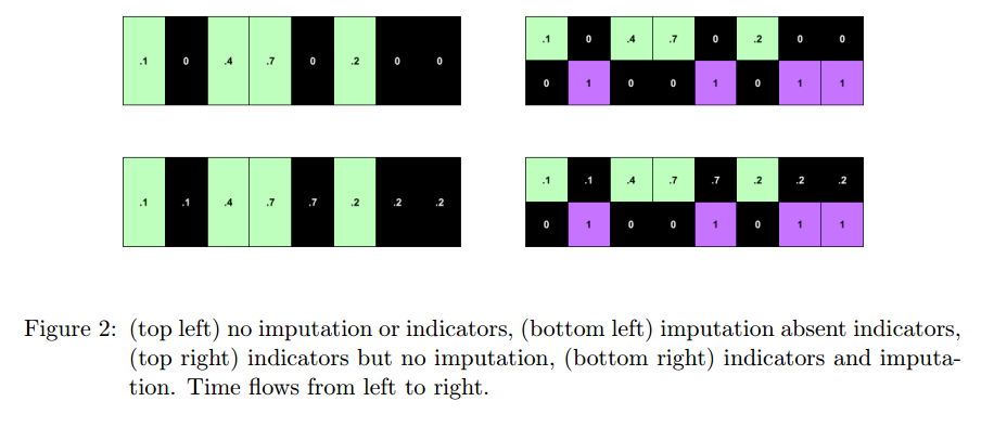
+ An RNN can learn about missing values and their importance only by using the indicator function. The nonlinearity from this type of model helps capturing these dependencies.
+ If one wants to use a linear model, feature engineering is needed to overcome its limitations.
+ indicator for whether a variable was measured at all
+ mean and standard deviation of the indicator
+ frequency with which a variable switches from measured to missing and vice-versa.
#### Architecture:
+ RNN with target replication following the work "Learning to Diagnose with LSTM Recurrent Neural Networks" by the same authors.
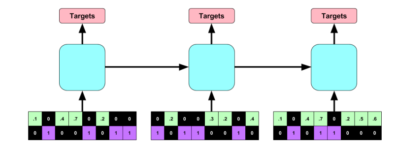
#### Dataset:
+ Children's Hospital LA
+ Episode is a multivariate time series that describes the stay of one patient in the intensive care unit
Dataset properties | Value
---------|----------
Number of episodes | 10,401
Duration of episodes | From 12h to several months
Time series variables | Systolic blood pressure, Diastolic blood pressure, Peripheral capillary refill rate, End tidal CO2, Fraction of inspired O2, Glasgow coma scale, Blood glucose, Heart rate, pH, Respiratory rate, Blood O2 Saturation, Body temperature, Urine output.
#### Experiments and Results:
**Goal**
+ Predict 128 diagnoses.
+ Multilabel: patients can have more than one diagnose.
**Methodology**
+ Split: 80% training, 10% validation, 10% test.
+ Normalized data to be in the range [0,1].
+ LSTM RNN:
+ 2 hidden layers with 128 cells. Dropout = 0.5, L2-regularization: 1e-6
+ Training for 100 epochs. Parameters chosen correspond to the time that generated the smallest error in the validation dataset.
+ Baselines:
+ Logistic Regression (L2 regularization)
+ MLP with 3 hidden layers and 500 hidden neurons / layer (parameters chosen via validation set)
+ Tested with raw-features and hand-engineered features.
+ Strategies for missing values:
+ Zeroing
+ Impute via forward / backfilling
+ Impute with zeros and use indicator function
+ Impute via forward / backfilling and use indicator function
+ Use indicator function only
#### Results
+ Metrics:
+ Micro AUC, Micro F1: calculated by adding the TPs, FPs, TNs and FNs for the entire dataset and for all classes.
+ Macro AUC, Macro F1: Arithmetic mean of AUCs and F1 scores for each of the classes.
+ Precision at 10: Fraction of correct diagnostics among the top 10 predictions of the model.
+ The upper bound for precision at 10 is 0.2281 since in the test set there are on average 2.281 diagnoses per patient.
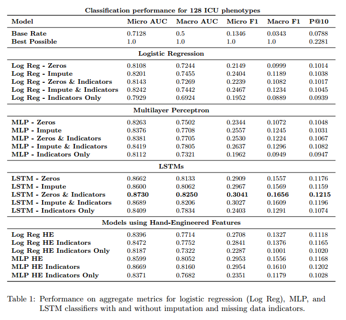
#### Discussion:
+ Predictive model based on data collected following a given routine. This routine can change if the model is put into practice. Will the model predictions in this new routine remain valid?
+ Missing values in a way give an indication of the type of treatment being followed.
+ Trade-off between complex models operating on raw features and very complex features operating on more interpretable models.
|

PVANet: Lightweight Deep Neural Networks for Real-time Object Detection
Sanghoon Hong and Byungseok Roh and Kye-Hyeon Kim and Yeongjae Cheon and Minje Park
arXiv e-Print archive - 2016 via Local arXiv
Keywords: cs.CV
First published: 2016/11/23 (7 years ago)
Abstract: In object detection, reducing computational cost is as important as improving accuracy for most practical usages. This paper proposes a novel network structure, which is an order of magnitude lighter than other state-of-the-art networks while maintaining the accuracy. Based on the basic principle of more layers with less channels, this new deep neural network minimizes its redundancy by adopting recent innovations including C.ReLU and Inception structure. We also show that this network can be trained efficiently to achieve solid results on well-known object detection benchmarks: 84.9% and 84.2% mAP on VOC2007 and VOC2012 while the required compute is less than 10% of the recent ResNet-101.
more
less
Sanghoon Hong and Byungseok Roh and Kye-Hyeon Kim and Yeongjae Cheon and Minje Park
arXiv e-Print archive - 2016 via Local arXiv
Keywords: cs.CV
First published: 2016/11/23 (7 years ago)
Abstract: In object detection, reducing computational cost is as important as improving accuracy for most practical usages. This paper proposes a novel network structure, which is an order of magnitude lighter than other state-of-the-art networks while maintaining the accuracy. Based on the basic principle of more layers with less channels, this new deep neural network minimizes its redundancy by adopting recent innovations including C.ReLU and Inception structure. We also show that this network can be trained efficiently to achieve solid results on well-known object detection benchmarks: 84.9% and 84.2% mAP on VOC2007 and VOC2012 while the required compute is less than 10% of the recent ResNet-101.
|
[link]
* They present a variation of Faster R-CNN.
* Faster R-CNN is a model that detects bounding boxes in images.
* Their variation is about as accurate as the best performing versions of Faster R-CNN.
* Their variation is significantly faster than these variations (roughly 50ms per image).
### How
* PVANET reuses the standard Faster R-CNN architecture:
* A base network that transforms an image into a feature map.
* A region proposal network (RPN) that uses the feature map to predict bounding box candidates.
* A classifier that uses the feature map and the bounding box candidates to predict the final bounding boxes.
* PVANET modifies the base network and keeps the RPN and classifier the same.
* Inception
* Their base network uses eight Inception modules.
* They argue that these are good choices here, because they are able to represent an image at different scales (aka at different receptive field sizes)
due to their mixture of 3x3 and 1x1 convolutions.
* 
* Representing an image at different scales is useful here in order to detect both large and small bounding boxes.
* Inception modules are also reasonably fast.
* Visualization of their Inception modules:
* 
* Concatenated ReLUs
* Before the eight Inception modules, they start the network with eight convolutions using concatenated ReLUs.
* These CReLUs compute both the classic ReLU result (`max(0, x)`) and concatenate to that the negated result, i.e. something like `f(x) = max(0, x <concat> (-1)*x)`.
* That is done, because among the early one can often find pairs of convolution filters that are the negated variations of each other.
So by adding CReLUs, the network does not have to compute these any more, instead they are created (almost) for free, reducing the computation time by up to 50%.
* Visualization of their final CReLU block:
* TODO
* 
* Multi-Scale output
* Usually one would generate the final feature map simply from the output of the last convolution.
* They instead combine the outputs of three different convolutions, each resembling a different scale (or level of abstraction).
* They take one from an early point of the network (downscaled), one from the middle part (kept the same) and one from the end (upscaled).
* They concatenate these and apply a 1x1 convolution to generate the final output.
* Other stuff
* Most of their network uses residual connections (including the Inception modules) to facilitate learning.
* They pretrain on ILSVRC2012 and then perform fine-tuning on MSCOCO, VOC 2007 and VOC 2012.
* They use plateau detection for their learning rate, i.e. if a moving average of the loss does not improve any more, they decrease the learning rate. They say that this increases accuracy significantly.
* The classifier in Faster R-CNN consists of fully connected layers. They compress these via Truncated SVD to speed things up. (That was already part of Fast R-CNN, I think.)
### Results
* On Pascal VOC 2012 they achieve 82.5% mAP at 46ms/image (Titan X GPU).
* Faster R-CNN + ResNet-101: 83.8% at 2.2s/image.
* Faster R-CNN + VGG16: 75.9% at 110ms/image.
* R-FCN + ResNet-101: 82.0% at 133ms/image.
* Decreasing the number of region proposals from 300 per image to 50 almost doubles the speed (to 27ms/image) at a small loss of 1.5 percentage points mAP.
* Using Truncated SVD for the classifier reduces the required timer per image by about 30% at roughly 1 percentage point of mAP loss.
|

R-FCN: Object Detection via Region-based Fully Convolutional Networks
Dai, Jifeng and Li, Yi and He, Kaiming and Sun, Jian
Neural Information Processing Systems Conference - 2016 via Local Bibsonomy
Keywords: dblp
Dai, Jifeng and Li, Yi and He, Kaiming and Sun, Jian
Neural Information Processing Systems Conference - 2016 via Local Bibsonomy
Keywords: dblp
|
[link]
* They present a variation of Faster R-CNN, i.e. a model that predicts bounding boxes in images and classifies them.
* In contrast to Faster R-CNN, their model is fully convolutional.
* In contrast to Faster R-CNN, the computation per bounding box candidate (region proposal) is very low.
### How
* The basic architecture is the same as in Faster R-CNN:
* A base network transforms an image to a feature map. Here they use ResNet-101 to do that.
* A region proposal network (RPN) uses the feature map to locate bounding box candidates ("region proposals") in the image.
* A classifier uses the feature map and the bounding box candidates and classifies each one of them into `C+1` classes,
where `C` is the number of object classes to spot (e.g. "person", "chair", "bottle", ...) and `1` is added for the background.
* During that process, small subregions of the feature maps (those that match the bounding box candidates) must be extracted and converted to fixed-sizes matrices.
The method to do that is called "Region of Interest Pooling" (RoI-Pooling) and is based on max pooling.
It is mostly the same as in Faster R-CNN.
* Visualization of the basic architecture:
* 
* Position-sensitive classification
* Fully convolutional bounding box detectors tend to not work well.
* The authors argue, that the problems come from the translation-invariance of convolutions, which is a desirable property in the case of classification but not when precise localization of objects is required.
* They tackle that problem by generating multiple heatmaps per object class, each one being slightly shifted ("position-sensitive score maps").
* More precisely:
* The classifier generates per object class `c` a total of `k*k` heatmaps.
* In the simplest form `k` is equal to `1`. Then only one heatmap is generated, which signals whether a pixel is part of an object of class `c`.
* They use `k=3*3`. The first of those heatmaps signals, whether a pixel is part of the *top left* corner of a bounding box of class `c`. The second heatmap signals, whether a pixel is part of the *top center* of a bounding box of class `c` (and so on).
* The RoI-Pooling is applied to these heatmaps.
* For `k=3*3`, each bounding box candidate is converted to `3*3` values. The first one resembles the top left corner of the bounding box candidate. Its value is generated by taking the average of the values in that area in the first heatmap.
* Once the `3*3` values are generated, the final score of class `c` for that bounding box candidate is computed by averaging the values.
* That process is repeated for all classes and a softmax is used to determine the final class.
* The graphic below shows examples for that:
* 
* The above described RoI-Pooling uses only averages and hence is almost (computationally) free.
* They make use of that during the training by sampling many candidates and only backpropagating on those with high losses (online hard example mining, OHEM).
* À trous trick
* In order to increase accuracy for small bounding boxes they use the à trous trick.
* That means that they use a pretrained base network (here ResNet-101), then remove a pooling layer and set the à trous rate (aka dilation) of all convolutions after the removed pooling layer to `2`.
* The á trous rate describes the distance of sampling locations of a convolution. Usually that is `1` (sampled locations are right next to each other). If it is set to `2`, there is one value "skipped" between each pair of neighbouring sampling location.
* By doing that, the convolutions still behave as if the pooling layer existed (and therefore their weights can be reused). At the same time, they work at an increased resolution, making them more capable of classifying small objects. (Runtime increases though.)
* Training of R-FCN happens similarly to Faster R-CNN.
### Results
* Similar accuracy as the most accurate Faster R-CNN configurations at a lower runtime of roughly 170ms per image.
* Switching to ResNet-50 decreases accuracy by about 2 percentage points mAP (at faster runtime). Switching to ResNet-152 seems to provide no measureable benefit.
* OHEM improves mAP by roughly 2 percentage points.
* À trous trick improves mAP by roughly 2 percentage points.
* Training on `k=1` (one heatmap per class) results in a failure, i.e. a model that fails to predict bounding boxes. `k=7` is slightly more accurate than `k=3`.
1 Comments
 |
Instance Normalization: The Missing Ingredient for Fast Stylization
Dmitry Ulyanov and Andrea Vedaldi and Victor Lempitsky
arXiv e-Print archive - 2016 via Local arXiv
Keywords: cs.CV
First published: 2016/07/27 (7 years ago)
Abstract: It this paper we revisit the fast stylization method introduced in Ulyanov et. al. (2016). We show how a small change in the stylization architecture results in a significant qualitative improvement in the generated images. The change is limited to swapping batch normalization with instance normalization, and to apply the latter both at training and testing times. The resulting method can be used to train high-performance architectures for real-time image generation. The code will is made available on github.
more
less
Dmitry Ulyanov and Andrea Vedaldi and Victor Lempitsky
arXiv e-Print archive - 2016 via Local arXiv
Keywords: cs.CV
First published: 2016/07/27 (7 years ago)
Abstract: It this paper we revisit the fast stylization method introduced in Ulyanov et. al. (2016). We show how a small change in the stylization architecture results in a significant qualitative improvement in the generated images. The change is limited to swapping batch normalization with instance normalization, and to apply the latter both at training and testing times. The resulting method can be used to train high-performance architectures for real-time image generation. The code will is made available on github.
|
[link]
* Style transfer between images works - in its original form - by iteratively making changes to a content image, so that its style matches more and more the style of a chosen style image.
* That iterative process is very slow.
* Alternatively, one can train a single feed-forward generator network to apply a style in one forward pass. The network is trained on a dataset of input images and their stylized versions (stylized versions can be generated using the iterative approach).
* So far, these generator networks were much faster than the iterative approach, but their quality was lower.
* They describe a simple change to these generator networks to increase the image quality (up to the same level as the iterative approach).
### How
* In the generator networks, they simply replace all batch normalization layers with instance normalization layers.
* Batch normalization normalizes using the information from the whole batch, while instance normalization normalizes each feature map on its own.
* Equations
* Let `H` = Height, `W` = Width, `T` = Batch size
* Batch Normalization:
* 
* Instance Normalization
* 
* They apply instance normalization at test time too (identically).
### Results
* Same image quality as iterative approach (at a fraction of the runtime).
* One content image with two different styles using their approach:
* 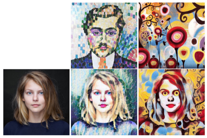
|
Stacked Hourglass Networks for Human Pose Estimation
Alejandro Newell and Kaiyu Yang and Jia Deng
arXiv e-Print archive - 2016 via Local arXiv
Keywords: cs.CV
First published: 2016/03/22 (8 years ago)
Abstract: This work introduces a novel Convolutional Network architecture for the task of human pose estimation. Features are processed across all scales and consolidated to best capture the various spatial relationships associated with the body. We show how repeated bottom-up, top-down processing used in conjunction with intermediate supervision is critical to improving the performance of the network. We refer to the architecture as a 'stacked hourglass' network based on the successive steps of pooling and upsampling that are done to produce a final set of estimates. State-of-the-art results are achieved on the FLIC and MPII benchmarks outcompeting all recent methods.
more
less
Alejandro Newell and Kaiyu Yang and Jia Deng
arXiv e-Print archive - 2016 via Local arXiv
Keywords: cs.CV
First published: 2016/03/22 (8 years ago)
Abstract: This work introduces a novel Convolutional Network architecture for the task of human pose estimation. Features are processed across all scales and consolidated to best capture the various spatial relationships associated with the body. We show how repeated bottom-up, top-down processing used in conjunction with intermediate supervision is critical to improving the performance of the network. We refer to the architecture as a 'stacked hourglass' network based on the successive steps of pooling and upsampling that are done to produce a final set of estimates. State-of-the-art results are achieved on the FLIC and MPII benchmarks outcompeting all recent methods.
|
[link]
Official code: https://github.com/anewell/pose-hg-train
* They suggest a new model architecture for human pose estimation (i.e. "lay a skeleton over a person").
* Their architecture is based progressive pooling followed by progressive upsampling, creating an hourglass form.
* Input are images showing a person's body.
* Outputs are K heatmaps (for K body joints), with each heatmap showing the likely position of a single joint on the person (e.g. "akle", "wrist", "left hand", ...).
### How
* *Basic building block*
* They use residuals as their basic building block.
* Each residual has three layers: One 1x1 convolution for dimensionality reduction (from 256 to 128 channels), a 3x3 convolution, a 1x1 convolution for dimensionality increase (back to 256).
* Visualized:
* 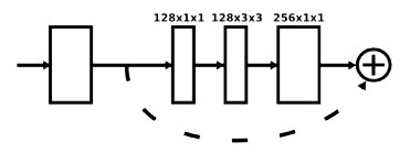
* *Architecture*
* Their architecture starts with one standard 7x7 convolutions that has strides of (2, 2).
* They use MaxPooling (2x2, strides of (2, 2)) to downsample the images/feature maps.
* They use Nearest Neighbour upsampling (factor 2) to upsample the images/feature maps.
* After every pooling step they add three of their basic building blocks.
* Before each pooling step they branch off the current feature map as a minor branch and apply three basic building blocks to it. Then they add it back to the main branch after that one has been upsampeled again to the original size.
* The feature maps between each basic building block have (usually) 256 channels.
* Their HourGlass ends in two 1x1 convolutions that create the heatmaps.
* They stack two of their HourGlass networks after each other. Between them they place an intermediate loss. That way, the second network can learn to improve the predictions of the first network.
* Architecture visualized:
* 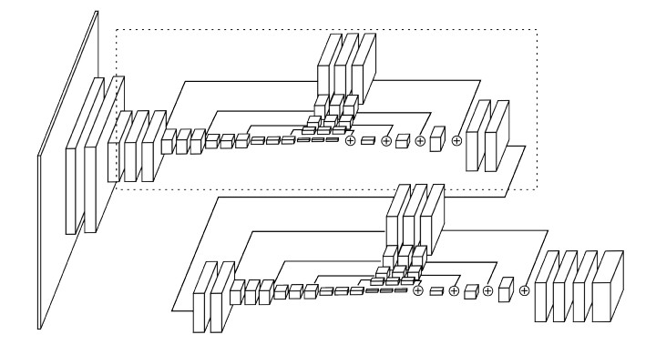
* *Heatmaps*
* The output generated by the network are heatmaps, one per joint.
* Each ground truth heatmap has a small gaussian peak at the correct position of a joint, everything else has value 0.
* If a joint isn't visible, the ground truth heatmap for that joint is all zeros.
* *Other stuff*
* They use batch normalization.
* Activation functions are ReLUs.
* They use RMSprob as their optimizer.
* Implemented in Torch.
### Results
* They train and test on FLIC (only one HourGlass) and MPII (two stacked HourGlass networks).
* Training is done with augmentations (horizontal flip, up to 30 degress rotation, scaling, no translation to keep the body of interest in the center of the image).
* Evaluation is done via PCK@0.2 (i.e. percentage of predicted keypoints that are within 0.2 head sizes of their ground truth annotation (head size of the specific body)).
* Results on FLIC are at >95%.
* Results on MPII are between 80.6% (ankle) and 97.6% (head). Average is 89.4%.
* Using two stacked HourGlass networks performs around 3% better than one HourGlass network (even when adjusting for parameters).
* Training time was 5 days on a Titan X (9xx generation).
|
Character-based Neural Machine Translation
Costa-Jussà, Marta R. and Fonollosa, José A. R.
Association for Computational Linguistics - 2016 via Local Bibsonomy
Keywords: dblp
Costa-Jussà, Marta R. and Fonollosa, José A. R.
Association for Computational Linguistics - 2016 via Local Bibsonomy
Keywords: dblp
|
[link]
* Most neural machine translation models currently operate on word vectors or one hot vectors of words.
* They instead generate the vector of each word on a character-level.
* Thereby, the model can spot character-similarities between words and treat them in a similar way.
* They do that only for the source language, not for the target language.
### How
* They treat each word of the source text on its own.
* To each word they then apply the model from [Character-aware neural language models](https://arxiv.org/abs/1508.06615), i.e. they do per word:
* Embed each character into a 620-dimensional space.
* Stack these vectors next to each other, resulting in a 2d-tensor in which each column is one of the vectors (i.e. shape `620xN` for `N` characters).
* Apply convolutions of size `620xW` to that tensor, where a few different values are used for `W` (i.e. some convolutions cover few characters, some cover many characters).
* Apply a tanh after these convolutions.
* Apply a max-over-time to the results of the convolutions, i.e. for each convolution use only the maximum value.
* Reshape to 1d-vector.
* Apply two highway-layers.
* They get 1024-dimensional vectors (one per word).
* Visualization of their steps:
* 
* Afterwards they apply the model from [Neural Machine Translation by Jointly Learning to Align and Translate](https://arxiv.org/abs/1409.0473) to these vectors, yielding a translation to a target language.
* Whenever that translation yields an unknown target-language-word ("UNK"), they replace it with the respective (untranslated) word from the source text.
### Results
* They the German-English [WMT](http://www.statmt.org/wmt15/translation-task.html) dataset.
* BLEU improvemements (compared to neural translation without character-level words):
* German-English improves by about 1.5 points.
* English-German improves by about 3 points.
* Reduction in the number of unknown target-language-words (same baseline again):
* German-English goes down from about 1500 to about 1250.
* English-German goes down from about 3150 to about 2650.
* Translation examples (Phrase = phrase-based/non-neural translation, NN = non-character-based neural translation, CHAR = theirs):
* 
|
HyperFace: A Deep Multi-task Learning Framework for Face Detection, Landmark Localization, Pose Estimation, and Gender Recognition
Ranjan, Rajeev and Patel, Vishal M. and Chellappa, Rama
arXiv e-Print archive - 2016 via Local Bibsonomy
Keywords: dblp
Ranjan, Rajeev and Patel, Vishal M. and Chellappa, Rama
arXiv e-Print archive - 2016 via Local Bibsonomy
Keywords: dblp
|
[link]
* They suggest a single architecture that tries to solve the following tasks:
* Face localization ("Where are faces in the image?")
* Face landmark localization ("For a given face, where are its landmarks, e.g. eyes, nose and mouth?")
* Face landmark visibility estimation ("For a given face, which of its landmarks are actually visible and which of them are occluded by other objects/people?")
* Face roll, pitch and yaw estimation ("For a given face, what is its rotation on the x/y/z-axis?")
* Face gender estimation ("For a given face, which gender does the person have?")
### How
* *Pretraining the base model*
* They start with a basic model following the architecture of AlexNet.
* They train that model to classify whether the input images are faces or not faces.
* They then remove the fully connected layers, leaving only the convolutional layers.
* *Locating bounding boxes of face candidates*
* They then use a [selective search and segmentation algorithm](https://www.robots.ox.ac.uk/~vgg/rg/papers/sande_iccv11.pdf) on images to extract bounding boxes of objects.
* Each bounding box is considered a possible face.
* Each bounding box is rescaled to 227x227.
* *Feature extraction per face candidate*
* They feed each bounding box through the above mentioned pretrained network.
* They extract the activations of the network from the layers `max1` (27x27x96), `conv3` (13x13x384) and `pool5` (6x6x256).
* They apply to the first two extracted tensors (from max1, conv3) convolutions so that their tensor shapes are reduced to 6x6xC.
* They concatenate the three tensors to a 6x6x768 tensor.
* They apply a 1x1 convolution to that tensor to reduce it to 6x6x192.
* They feed the result through a fully connected layer resulting in 3072-dimensional vectors (per face candidate).
* *Classification and regression*
* They feed each 3072-dimensional vector through 5 separate networks:
1. Detection: Does the bounding box contain a face or no face. (2 outputs, i.e. yes/no)
2. Landmark Localization: What are the coordinates of landmark features (e.g. mouth, nose, ...). (21 landmarks, each 2 values for x/y = 42 outputs total)
3. Landmark Visibility: Which landmarks are visible. (21 yes/no outputs)
4. Pose estimation: Roll, pitch, yaw of the face. (3 outputs)
5. Gender estimation: Male/female face. (2 outputs)
* Each of these network contains a single fully connected layer with 512 nodes, followed by the output layer with the above mentioned number of nodes.
* *Architecture Visualization*:
* 
* *Training*
* The base model is trained once (see above).
* The feature extraction layers and the five classification/regression networks are trained afterwards (jointly).
* The loss functions for the five networks are:
1. Detection: BCE (binary cross-entropy). Detected bounding boxes that have an overlap `>=0.5` with an annotated face are considered positive samples, bounding boxes with overlap `<0.35` are considered negative samples, everything in between is ignored.
2. Landmark localization: Roughly MSE (mean squared error), with some weighting for visibility. Only bounding boxes with overlap `>0.35` are considered. Coordinates are normalized with respect to the bounding boxes center, width and height.
3. Landmark visibility: MSE (predicted visibility factor vs. expected visibility factor). Only for bounding boxes with overlap `>0.35`.
4. Pose estimation: MSE.
5. Gender estimation: BCE.
* *Testing*
* They use two postprocessing methods for detected faces:
* Iterative Region Proposals:
* They localize landmarks per face region.
* Then they compute a more appropriate face bounding box based on the localized landmarks.
* They feed that new bounding box through the network.
* They compute the face score (face / not face, i.e. number between 0 and 1) for both bounding boxes and choose the one with the higher score.
* This shrinks down bounding boxes that turned out to be too big.
* The method visualized:
* 
* Landmarks-based Non-Maximum Suppression:
* When multiple detected face bounding boxes overlap, one has to choose which of them to keep.
* A method to do that is to only keep the bounding box with the highest face-score.
* They instead use a median-of-k method.
* Their steps are:
1. Reduce every box in size so that it is a bounding box around the localized landmarks.
2. For every box, find all bounding boxes with a certain amount of overlap.
3. Among these bounding boxes, select the `k` ones with highest face score.
4. Based on these boxes, create a new box which's size is derived from the median coordinates of the landmarks.
5. Compute the median values for landmark coordinates, landmark visibility, gender, pose and use it as the respective values for the new box.
### Results
* Example results:
* 
* They test on AFW, AFWL, PASCAL, FDDB, CelebA.
* They achieve the best mean average precision values on PASCAL and AFW (compared to selected competitors).
* AFW results visualized:
* 
* Their approach achieve good performance on FDDB. It has some problems with small and/or blurry faces.
* If the feature fusion is removed from their approach (i.e. extracting features only from one fully connected layer at the end of the base network instead of merging feature maps from different convolutional layers), the accuracy of the predictions goes down.
* Their architecture ends in 5 shallow networks and shares many layers before them. If instead these networks share no or few layers, the accuracy of the predictions goes down.
* The postprocessing of bounding boxes (via Iterative Region Proposals and Landmarks-based Non-Maximum Suppression) has a quite significant influence on the performance.
* Processing time per image is 3s, of which 2s is the selective search algorithm (for the bounding boxes).
|
Face attribute prediction using off-the-shelf CNN features
Zhong, Yang and Sullivan, Josephine and Li, Haibo
IEEE ICB - 2016 via Local Bibsonomy
Keywords: dblp
Zhong, Yang and Sullivan, Josephine and Li, Haibo
IEEE ICB - 2016 via Local Bibsonomy
Keywords: dblp
|
[link]
* When using pretrained networks (like VGG) to solve tasks, one has to use features generated by these networks.
* These features come from specific layers, e.g. from the fully connected layers at the end of the network.
* They test whether the features from fully connected layers or from the last convolutional layer are better suited for face attribute prediction.
### How
* Base networks
* They use standard architectures for their test networks, specifically the architectures of FaceNet and VGG (very deep version).
* They modify these architectures to both use PReLUs.
* They do not use the pretrained weights, instead they train the networks on their own.
* They train them on the WebFace dataset (350k images, 10k different identities) to classify the identity of the shown person.
* Attribute prediction
* After training of the base networks, they train a separate SVM to predict attributes of faces.
* The datasets used for this step are CelebA (100k images, 10k identities) and LFWA (13k images, 6k identities).
* Each image in these datasets is annotated with 40 binary face attributes.
* Examples for attributes: Eyeglasses, bushy eyebrows, big lips, ...
* The features for the SVM are extracted from the base networks (i.e. feed forward a face through the network, then take the activations of a specific layer).
* The following features are tested:
* FC2: Activations of the second fully connected layer of the base network.
* FC1: As FC2, but the first fully connected layer.
* Spat 3x3: Activations of the last convolutional layer, max-pooled so that their widths and heights are both 3 (i.e. shape Cx3x3).
* Spat 1x1: Same as "Spat 3x3", but max-pooled to Cx1x1.
### Results
* The SVMs trained on "Spat 1x1" performed overall worst, the ones trained on "Spat 3x3" performed best.
* The accuracy order was roughly: `Spat 3x3 > FC1 > FC2 > Spat 1x1`.
* This effect was consistent for both networks (VGG, FaceNet) and for other training datasets as well.
* FC2 performed particularly bad for the "blurry" attribute (most likely because that was unimportant to the classification task).
* Accuracy comparison per attribute:
* 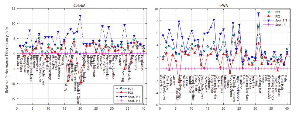
* The conclusion is, that when using pretrained networks one should not only try the last fully connected layer. Many characteristics of the input image might not appear any more in that layer (and later ones in general) as they were unimportant to the classification task.
|
CMS-RCNN: Contextual Multi-Scale Region-based CNN for Unconstrained Face Detection
Zhu, Chenchen and Zheng, Yutong and Luu, Khoa and Savvides, Marios
arXiv e-Print archive - 2016 via Local Bibsonomy
Keywords: dblp
Zhu, Chenchen and Zheng, Yutong and Luu, Khoa and Savvides, Marios
arXiv e-Print archive - 2016 via Local Bibsonomy
Keywords: dblp
|
[link]
* They describe a model to locate faces in images.
* Their model uses information from suspected face regions *and* from the corresponding suspected body regions to classify whether a region contains a face.
* The intuition is, that seeing the region around the face (specifically where the body should be) can help in estimating whether a suspected face is really a face (e.g. it might also be part of a painting, statue or doll).
### How
* Their whole model is called "CMS-RCNN" (Contextual Multi-Scale Region-CNN).
* It is based on the "Faster R-CNN" architecture.
* It uses the VGG network.
* Subparts of their model are: MS-RPN, CMS-CNN.
* MS-RPN finds candidate face regions. CMS-CNN refines their bounding boxes and classifies them (face / not face).
* **MS-RPN** (Multi-Scale Region Proposal Network)
* "Looks" at the feature maps of the network (VGG) at multiple scales (i.e. before/after pooling layers) and suggests regions for possible faces.
* Steps:
* Feed an image through the VGG network.
* Extract the feature maps of the three last convolutions that are before a pooling layer.
* Pool these feature maps so that they have the same heights and widths.
* Apply L2 normalization to each feature map so that they all have the same scale.
* Apply a 1x1 convolution to merge them to one feature map.
* Regress face bounding boxes from that feature map according to the Faster R-CNN technique.
* **CMS-CNN** (Contextual Multi-Scale CNN):
* "Looks" at feature maps of face candidates found by MS-RPN and classifies whether these regions contains faces.
* It also uses the same multi-scale technique (i.e. take feature maps from convs before pooling layers).
* It uses some area around these face regions as additional information (suspected regions of bodies).
* Steps:
* Receive face candidate regions from MS-RPN.
* Do per candidate region:
* Calculate the suspected coordinates of the body (only based on the x/y-position and size of the face region, i.e. not learned).
* Extract the feature maps of the *face* region (at multiple scales) and apply RoI-Pooling to it (i.e. convert to a fixed height and width).
* Extract the feature maps of the *body* region (at multiple scales) and apply RoI-Pooling to it (i.e. convert to a fixed height and width).
* L2-normalize each feature map.
* Concatenate the (RoI-pooled and normalized) feature maps of the face (at multiple scales) with each other (creates one tensor).
* Concatenate the (RoI-pooled and normalized) feature maps of the body (at multiple scales) with each other (creates another tensor).
* Apply a 1x1 convolution to the face tensor.
* Apply a 1x1 convolution to the body tensor.
* Apply two fully connected layers to the face tensor, creating a vector.
* Apply two fully connected layers to the body tensor, creating a vector.
* Concatenate both vectors.
* Based on that vector, make a classification of whether it is really a face.
* Based on that vector, make a regression of the face's final bounding box coordinates and dimensions.
* Note: They use in both networks the multi-scale approach in order to be able to find small or tiny faces. Otherwise, after pooling these small faces would be hard or impossible to detect.
### Results
* Adding context to the classification (i.e. the body regions) empirically improves the results.
* Their model achieves the highest recall rate on FDDB compared to other models. However, it has lower recall if only very few false positives are accepted.
* FDDB ROC curves (theirs is bold red):
* 
* Example results on FDDB:
* 
|
InfoGAN: Interpretable Representation Learning by Information Maximizing Generative Adversarial Nets
Chen, Xi and Chen, Xi and Duan, Yan and Houthooft, Rein and Schulman, John and Sutskever, Ilya and Abbeel, Pieter
Neural Information Processing Systems Conference - 2016 via Local Bibsonomy
Keywords: dblp
Chen, Xi and Chen, Xi and Duan, Yan and Houthooft, Rein and Schulman, John and Sutskever, Ilya and Abbeel, Pieter
Neural Information Processing Systems Conference - 2016 via Local Bibsonomy
Keywords: dblp
|
[link]
* Usually GANs transform a noise vector `z` into images. `z` might be sampled from a normal or uniform distribution.
* The effect of this is, that the components in `z` are deeply entangled.
* Changing single components has hardly any influence on the generated images. One has to change multiple components to affect the image.
* The components end up not being interpretable. Ideally one would like to have meaningful components, e.g. for human faces one that controls the hair length and a categorical one that controls the eye color.
* They suggest a change to GANs based on Mutual Information, which leads to interpretable components.
* E.g. for MNIST a component that controls the stroke thickness and a categorical component that controls the digit identity (1, 2, 3, ...).
* These components are learned in a (mostly) unsupervised fashion.
### How
* The latent code `c`
* "Normal" GANs parameterize the generator as `G(z)`, i.e. G receives a noise vector and transforms it into an image.
* This is changed to `G(z, c)`, i.e. G now receives a noise vector `z` and a latent code `c` and transforms both into an image.
* `c` can contain multiple variables following different distributions, e.g. in MNIST a categorical variable for the digit identity and a gaussian one for the stroke thickness.
* Mutual Information
* If using a latent code via `G(z, c)`, nothing forces the generator to actually use `c`. It can easily ignore it and just deteriorate to `G(z)`.
* To prevent that, they force G to generate images `x` in a way that `c` must be recoverable. So, if you have an image `x` you must be able to reliable tell which latent code `c` it has, which means that G must use `c` in a meaningful way.
* This relationship can be expressed with mutual information, i.e. the mutual information between `x` and `c` must be high.
* The mutual information between two variables X and Y is defined as `I(X; Y) = entropy(X) - entropy(X|Y) = entropy(Y) - entropy(Y|X)`.
* If the mutual information between X and Y is high, then knowing Y helps you to decently predict the value of X (and the other way round).
* If the mutual information between X and Y is low, then knowing Y doesn't tell you much about the value of X (and the other way round).
* The new GAN loss becomes `old loss - lambda * I(G(z, c); c)`, i.e. the higher the mutual information, the lower the result of the loss function.
* Variational Mutual Information Maximization
* In order to minimize `I(G(z, c); c)`, one has to know the distribution `P(c|x)` (from image to latent code), which however is unknown.
* So instead they create `Q(c|x)`, which is an approximation of `P(c|x)`.
* `I(G(z, c); c)` is then computed using a lower bound maximization, similar to the one in variational autoencoders (called "Variational Information Maximization", hence the name "InfoGAN").
* Basic equation: `LowerBoundOfMutualInformation(G, Q) = E[log Q(c|x)] + H(c) <= I(G(z, c); c)`
* `c` is the latent code.
* `x` is the generated image.
* `H(c)` is the entropy of the latent codes (constant throughout the optimization).
* Optimization w.r.t. Q is done directly.
* Optimization w.r.t. G is done via the reparameterization trick.
* If `Q(c|x)` approximates `P(c|x)` *perfectly*, the lower bound becomes the mutual information ("the lower bound becomes tight").
* In practice, `Q(c|x)` is implemented as a neural network. Both Q and D have to process the generated images, which means that they can share many convolutional layers, significantly reducing the extra cost of training Q.
### Results
* MNIST
* They use for `c` one categorical variable (10 values) and two continuous ones (uniform between -1 and +1).
* InfoGAN learns to associate the categorical one with the digit identity and the continuous ones with rotation and width.
* Applying Q(c|x) to an image and then classifying only on the categorical variable (i.e. fully unsupervised) yields 95% accuracy.
* Sampling new images with exaggerated continuous variables in the range `[-2,+2]` yields sound images (i.e. the network generalizes well).
* 
* 3D face images
* InfoGAN learns to represent the faces via pose, elevation, lighting.
* They used five uniform variables for `c`. (So two of them apparently weren't associated with anything sensible? They are not mentioned.)
* 3D chair images
* InfoGAN learns to represent the chairs via identity (categorical) and rotation or width (apparently they did two experiments).
* They used one categorical variable (four values) and one continuous variable (uniform `[-1, +1]`).
* SVHN
* InfoGAN learns to represent lighting and to spot the center digit.
* They used four categorical variables (10 values each) and two continuous variables (uniform `[-1, +1]`). (Again, a few variables were apparently not associated with anything sensible?)
* CelebA
* InfoGAN learns to represent pose, presence of sunglasses (not perfectly), hair style and emotion (in the sense of "smiling or not smiling").
* They used 10 categorical variables (10 values each). (Again, a few variables were apparently not associated with anything sensible?)
* 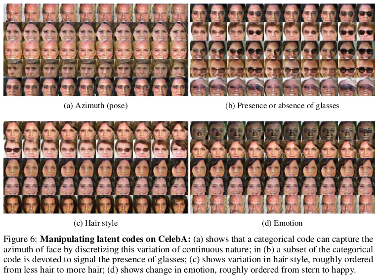
|
FractalNet: Ultra-Deep Neural Networks without Residuals
Larsson, Gustav and Maire, Michael and Shakhnarovich, Gregory
arXiv e-Print archive - 2016 via Local Bibsonomy
Keywords: dblp
Larsson, Gustav and Maire, Michael and Shakhnarovich, Gregory
arXiv e-Print archive - 2016 via Local Bibsonomy
Keywords: dblp
|
[link]
* They describe an architecture for deep CNNs that contains short and long paths. (Short = few convolutions between input and output, long = many convolutions between input and output)
* They achieve comparable accuracy to residual networks, without using residuals.
### How
* Basic principle:
* They start with two branches. The left branch contains one convolutional layer, the right branch contains a subnetwork.
* That subnetwork again contains a left branch (one convolutional layer) and a right branch (a subnetwork).
* This creates a recursion.
* At the last step of the recursion they simply insert two convolutional layers as the subnetwork.
* Each pair of branches (left and right) is merged using a pair-wise mean. (Result: One of the branches can be skipped or removed and the result after the merge will still be sound.)
* Their recursive expansion rule (left) and architecture (middle and right) visualized:

* Blocks:
* Each of the recursively generated networks is one block.
* They chain five blocks in total to create the network that they use for their experiments.
* After each block they add a max pooling layer.
* Their first block uses 64 filters per convolutional layer, the second one 128, followed by 256, 512 and again 512.
* Drop-path:
* They randomly dropout whole convolutional layers between merge-layers.
* They define two methods for that:
* Local drop-path: Drops each input to each merge layer with a fixed probability, but at least one always survives. (See image, first three examples.)
* Global drop-path: Drops convolutional layers so that only a single columns (and thereby path) in the whole network survives. (See image, right.)
* Visualization:
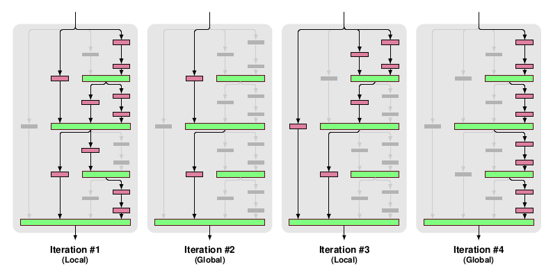
### Results
* They test on CIFAR-10, CIFAR-100 and SVHN with no or mild (crops, flips) augmentation.
* They add dropout at the start of each block (probabilities: 0%, 10%, 20%, 30%, 40%).
* They use for 50% of the batches local drop-path at 15% and for the other 50% global drop-path.
* They achieve comparable accuracy to ResNets (a bit behind them actually).
* Note: The best ResNet that they compare to is "ResNet with Identity Mappings". They don't compare to Wide ResNets, even though they perform best.
* If they use image augmentations, dropout and drop-path don't seem to provide much benefit (only small improvement).
* If they extract the deepest column and test on that one alone, they achieve nearly the same performance as with the whole network.
* They derive from that, that their fractal architecture is actually only really used to help that deepest column to learn anything. (Without shorter paths it would just learn nothing due to vanishing gradients.)
|
PlaNet - Photo Geolocation with Convolutional Neural Networks
Weyand, Tobias and Kostrikov, Ilya and Philbin, James
European Conference on Computer Vision - 2016 via Local Bibsonomy
Keywords: dblp
Weyand, Tobias and Kostrikov, Ilya and Philbin, James
European Conference on Computer Vision - 2016 via Local Bibsonomy
Keywords: dblp
|
[link]
* They describe a convolutional network that takes in photos and returns where (on the planet) these photos were likely made.
* The output is a distribution over locations around the world (so not just one single location). This can be useful in the case of ambiguous images.
### How
* Basic architecture
* They simply use the Inception architecture for their model.
* They have 97M parameters.
* Grid
* The network uses a grid of cells over the planet.
* For each photo and every grid cell it returns the likelihood that the photo was made within the region covered by the cell (simple softmax layer).
* The naive way would be to use a regular grid around the planet (i.e. a grid in which all cells have the same size).
* Possible disadvantages:
* In places where lots of photos are taken you still have the same grid cell size as in places where barely any photos are taken.
* Maps are often distorted towards the poles (countries are represented much larger than they really are). This will likely affect the grid cells too.
* They instead use an adaptive grid pattern based on S2 cells.
* S2 cells interpret the planet as a sphere and project a cube onto it.
* The 6 sides of the cube are then partitioned using quad trees, creating the grid cells.
* They don't use the same depth for all quad trees. Instead they subdivide them only if their leafs contain enough photos (based on their dataset of geolocated images).
* They remove some cells for which their dataset does not contain enough images, e.g. cells on oceans. (They also remove these images from the dataset. They don't say how many images are affected by this.)
* They end up with roughly 26k cells, some of them reaching the street level of major cities.
* Visualization of their cells:
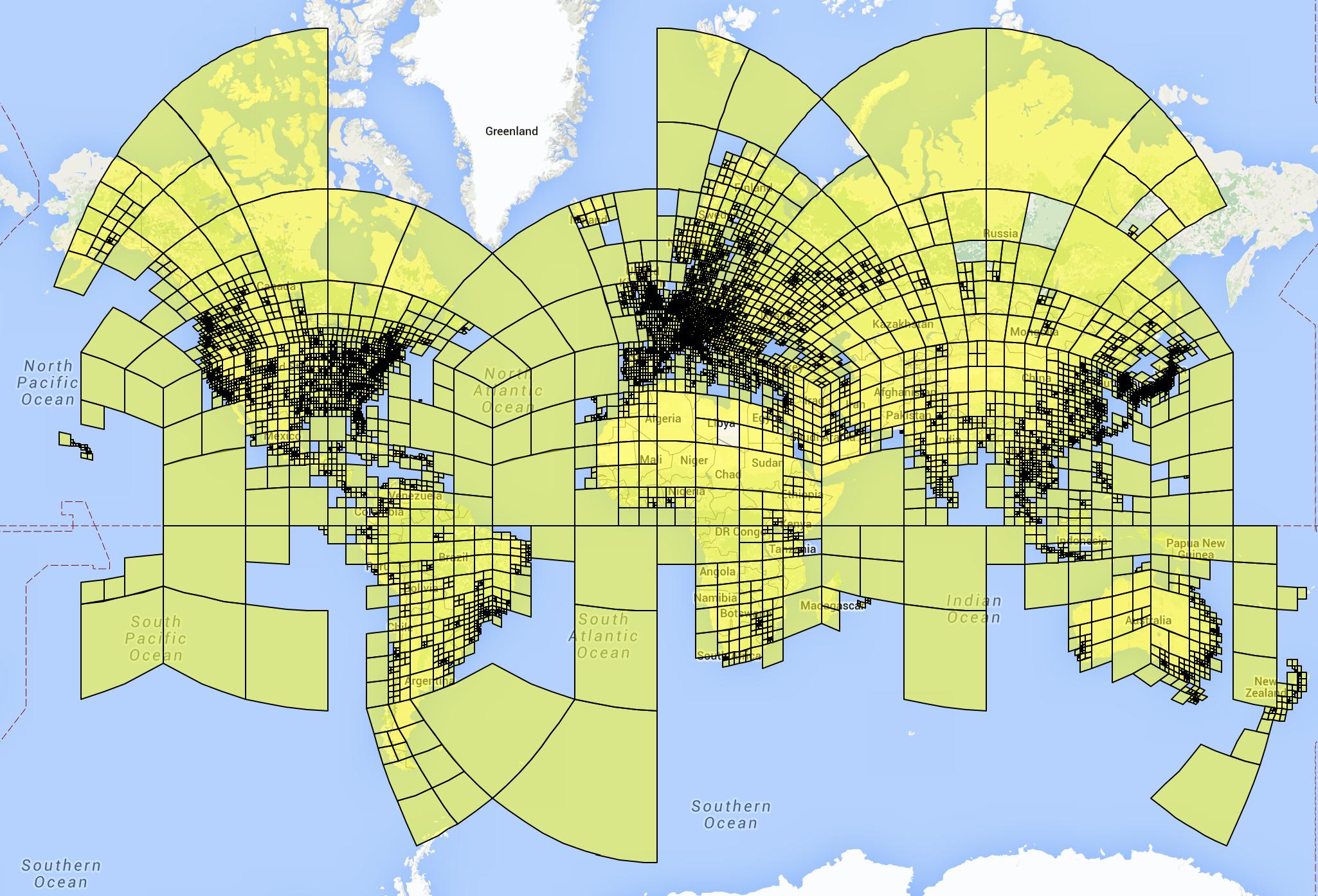
* Training
* For each example photo that they feed into the network, they set the correct grid cell to `1.0` and all other grid cells to `0.0`.
* They train on a dataset of 126M images with Exif geolocation information. The images were collected from all over the web.
* They used Adagrad.
* They trained on 200 CPUs for 2.5 months.
* Album network
* For photo albums they develop variations of their network.
* They do that because albums often contain images that are very hard to geolocate on their own, but much easier if the other images of the album are seen.
* They use LSTMs for their album network.
* The simplest one just iterates over every photo, applies their previously described model to it and extracts the last layer (before output) from that model. These vectors (one per image) are then fed into an LSTM, which is trained to predict (again) the grid cell location per image.
* More complicated versions use multiple passes or are bidirectional LSTMs (to use the information from the last images to classify the first ones in the album).
### Results
* They beat previous models (based on hand-engineered features or nearest neighbour methods) by a significant margin.
* In a small experiment they can beat experienced humans in geoguessr.com.
* Based on a dataset of 2.3M photos from Flickr, their method correctly predicts the country where the photo was made in 30% of all cases (top-1; top-5: about 50%). City-level accuracy is about 10% (top-1; top-5: about 18%).
* Example predictions (using in coarser grid with 354 cells):

* Using the LSTM-technique for albums significantly improves prediction accuracy for these images.
|
Generating images with recurrent adversarial networks
Daniel Jiwoong Im and Chris Dongjoo Kim and Hui Jiang and Roland Memisevic
arXiv e-Print archive - 2016 via Local arXiv
Keywords: cs.LG, cs.CV
First published: 2016/02/16 (8 years ago)
Abstract: Gatys et al. (2015) showed that optimizing pixels to match features in a convolutional network with respect reference image features is a way to render images of high visual quality. We show that unrolling this gradient-based optimization yields a recurrent computation that creates images by incrementally adding onto a visual "canvas". We propose a recurrent generative model inspired by this view, and show that it can be trained using adversarial training to generate very good image samples. We also propose a way to quantitatively compare adversarial networks by having the generators and discriminators of these networks compete against each other.
more
less
Daniel Jiwoong Im and Chris Dongjoo Kim and Hui Jiang and Roland Memisevic
arXiv e-Print archive - 2016 via Local arXiv
Keywords: cs.LG, cs.CV
First published: 2016/02/16 (8 years ago)
Abstract: Gatys et al. (2015) showed that optimizing pixels to match features in a convolutional network with respect reference image features is a way to render images of high visual quality. We show that unrolling this gradient-based optimization yields a recurrent computation that creates images by incrementally adding onto a visual "canvas". We propose a recurrent generative model inspired by this view, and show that it can be trained using adversarial training to generate very good image samples. We also propose a way to quantitatively compare adversarial networks by having the generators and discriminators of these networks compete against each other.
|
[link]
* What
* They describe a new architecture for GANs.
* The architecture is based on letting the Generator (G) create images in multiple steps, similar to DRAW.
* They also briefly suggest a method to compare the quality of the results of different generators with each other.
* How
* In a classic GAN one samples a noise vector `z`, feeds that into a Generator (`G`), which then generates an image `x`, which is then fed through the Discriminator (`D`) to estimate its quality.
* Their method operates in basically the same way, but internally G is changed to generate images in multiple time steps.
* Outline of how their G operates:
* Time step 0:
* Input: Empty image `delta C-1`, randomly sampled `z`.
* Feed `delta C-1` through a number of downsampling convolutions to create a tensor. (Not very useful here, as the image is empty. More useful in later timesteps.)
* Feed `z` through a number of upsampling convolutions to create a tensor (similar to DCGAN).
* Concat the output of the previous two steps.
* Feed that concatenation through a few more convolutions.
* Output: `delta C0` (changes to apply to the empty starting canvas).
* Time step 1 (and later):
* Input: Previous change `delta C0`, randomly sampled `z` (can be the same as in step 0).
* Feed `delta C0` through a number of downsampling convolutions to create a tensor.
* Feed `z` through a number of upsampling convolutions to create a tensor (similar to DCGAN).
* Concat the output of the previous two steps.
* Feed that concatenation through a few more convolutions.
* Output: `delta C1` (changes to apply to the empty starting canvas).
* At the end, after all timesteps have been performed:
* Create final output image by summing all the changes, i.e. `delta C0 + delta C1 + ...`, which basically means `empty start canvas + changes from time step 0 + changes from time step 1 + ...`.
* Their architecture as an image:
* 
* Comparison measure
* They suggest a new method to compare GAN results with each other.
* They suggest to train pairs of G and D, e.g. for two pairs (G1, D1), (G2, D2). Then they let the pairs compete with each other.
* To estimate the quality of D they suggest `r_test = errorRate(D1, testset) / errorRate(D2, testset)`. ("Which D is better at spotting that the test set images are real images?")
* To estimate the quality of the generated samples they suggest `r_sample = errorRate(D1, images by G2) / errorRate(D2, images by G1)`. ("Which G is better at fooling an unknown D, i.e. possibly better at generating life-like images?")
* They suggest to estimate which G is better using r_sample and then to estimate how valid that result is using r_test.
* Results
* Generated images of churches, with timesteps 1 to 5:
* 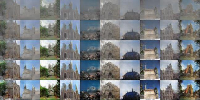
* Overfitting
* They saw no indication of overfitting in the sense of memorizing images from the training dataset.
* They however saw some indication of G just interpolating between some good images and of G reusing small image patches in different images.
* Randomness of noise vector `z`:
* Sampling the noise vector once seems to be better than resampling it at every timestep.
* Resampling it at every time step often led to very similar looking output images.
|
Adversarially Learned Inference
Vincent Dumoulin and Ishmael Belghazi and Ben Poole and Alex Lamb and Martin Arjovsky and Olivier Mastropietro and Aaron Courville
arXiv e-Print archive - 2016 via Local arXiv
Keywords: stat.ML, cs.LG
First published: 2016/06/02 (8 years ago)
Abstract: We introduce the adversarially learned inference (ALI) model, which jointly learns a generation network and an inference network using an adversarial process. The generation network maps samples from stochastic latent variables to the data space while the inference network maps training examples in data space to the space of latent variables. An adversarial game is cast between these two networks and a discriminative network that is trained to distinguish between joint latent/data-space samples from the generative network and joint samples from the inference network. We illustrate the ability of the model to learn mutually coherent inference and generation networks through the inspections of model samples and reconstructions and confirm the usefulness of the learned representations by obtaining a performance competitive with other recent approaches on the semi-supervised SVHN task.
more
less
Vincent Dumoulin and Ishmael Belghazi and Ben Poole and Alex Lamb and Martin Arjovsky and Olivier Mastropietro and Aaron Courville
arXiv e-Print archive - 2016 via Local arXiv
Keywords: stat.ML, cs.LG
First published: 2016/06/02 (8 years ago)
Abstract: We introduce the adversarially learned inference (ALI) model, which jointly learns a generation network and an inference network using an adversarial process. The generation network maps samples from stochastic latent variables to the data space while the inference network maps training examples in data space to the space of latent variables. An adversarial game is cast between these two networks and a discriminative network that is trained to distinguish between joint latent/data-space samples from the generative network and joint samples from the inference network. We illustrate the ability of the model to learn mutually coherent inference and generation networks through the inspections of model samples and reconstructions and confirm the usefulness of the learned representations by obtaining a performance competitive with other recent approaches on the semi-supervised SVHN task.
|
[link]
* They suggest a new architecture for GANs.
* Their architecture adds another Generator for a reverse branch (from images to noise vector `z`).
* Their architecture takes some ideas from VAEs/variational neural nets.
* Overall they can improve on the previous state of the art (DCGAN).
### How
* Architecture
* Usually, in GANs one feeds a noise vector `z` into a Generator (G), which then generates an image (`x`) from that noise.
* They add a reverse branch (G2), in which another Generator takes a real image (`x`) and generates a noise vector `z` from that.
* The noise vector can now be viewed as a latent space vector.
* Instead of letting G2 generate *discrete* values for `z` (as it is usually done), they instead take the approach commonly used VAEs and use *continuous* variables instead.
* That is, if `z` represents `N` latent variables, they let G2 generate `N` means and `N` variances of gaussian distributions, with each distribution representing one value of `z`.
* So the model could e.g. represent something along the lines of "this face looks a lot like a female, but with very low probability could also be male".
* Training
* The Discriminator (D) is now trained on pairs of either `(real image, generated latent space vector)` or `(generated image, randomly sampled latent space vector)` and has to tell them apart from each other.
* Both Generators are trained to maximally confuse D.
* G1 (from `z` to `x`) confuses D maximally, if it generates new images that (a) look real and (b) fit well to the latent variables in `z` (e.g. if `z` says "image contains a cat", then the image should contain a cat).
* G2 (from `x` to `z`) confuses D maximally, if it generates good latent variables `z` that fit to the image `x`.
* Continuous variables
* The variables in `z` follow gaussian distributions, which makes the training more complicated, as you can't trivially backpropagate through gaussians.
* When training G1 (from `z` to `x`) the situation is easy: You draw a random `z`-vector following a gaussian distribution (`N(0, I)`). (This is basically the same as in "normal" GANs. They just often use uniform distributions instead.)
* When training G2 (from `x` to `z`) the situation is a bit harder.
* Here we need to use the reparameterization trick here.
* That roughly means, that G2 predicts the means and variances of the gaussian variables in `z` and then we draw a sample of `z` according to exactly these means and variances.
* That sample gives us discrete values for our backpropagation.
* If we do that sampling often enough, we get a good approximation of the true gradient (of the continuous variables). (Monte Carlo approximation.)
* Results
* Images generated based on Celeb-A dataset:
* 
* Left column per pair: Real image, right column per pair: reconstruction (`x -> z` via G2, then `z -> x` via G1)
* 
* Reconstructions of SVHN, notice how the digits often stay the same, while the font changes:
* 
* CIFAR-10 samples, still lots of errors, but some quite correct:
* 
|
Rank Ordered Autoencoders
Paul Bertens
arXiv e-Print archive - 2016 via Local arXiv
Keywords: cs.LG, stat.ML, I.2.6; I.5.1; I.4.2
First published: 2016/05/05 (8 years ago)
Abstract: A new method for the unsupervised learning of sparse representations using autoencoders is proposed and implemented by ordering the output of the hidden units by their activation value and progressively reconstructing the input in this order. This can be done efficiently in parallel with the use of cumulative sums and sorting only slightly increasing the computational costs. Minimizing the difference of this progressive reconstruction with respect to the input can be seen as minimizing the number of active output units required for the reconstruction of the input. The model thus learns to reconstruct optimally using the least number of active output units. This leads to high sparsity without the need for extra hyperparameters, the amount of sparsity is instead implicitly learned by minimizing this progressive reconstruction error. Results of the trained model are given for patches of the CIFAR10 dataset, showing rapid convergence of features and extremely sparse output activations while maintaining a minimal reconstruction error and showing extreme robustness to overfitting. Additionally the reconstruction as function of number of active units is presented which shows the autoencoder learns a rank order code over the input where the highest ranked units correspond to the highest decrease in reconstruction error.
more
less
Paul Bertens
arXiv e-Print archive - 2016 via Local arXiv
Keywords: cs.LG, stat.ML, I.2.6; I.5.1; I.4.2
First published: 2016/05/05 (8 years ago)
Abstract: A new method for the unsupervised learning of sparse representations using autoencoders is proposed and implemented by ordering the output of the hidden units by their activation value and progressively reconstructing the input in this order. This can be done efficiently in parallel with the use of cumulative sums and sorting only slightly increasing the computational costs. Minimizing the difference of this progressive reconstruction with respect to the input can be seen as minimizing the number of active output units required for the reconstruction of the input. The model thus learns to reconstruct optimally using the least number of active output units. This leads to high sparsity without the need for extra hyperparameters, the amount of sparsity is instead implicitly learned by minimizing this progressive reconstruction error. Results of the trained model are given for patches of the CIFAR10 dataset, showing rapid convergence of features and extremely sparse output activations while maintaining a minimal reconstruction error and showing extreme robustness to overfitting. Additionally the reconstruction as function of number of active units is presented which shows the autoencoder learns a rank order code over the input where the highest ranked units correspond to the highest decrease in reconstruction error.
|
[link]
  * Autoencoders typically have some additional criterion that pushes them towards learning meaningful representations.
    * E.g. L1-Penalty on the code layer (z), Dropout on z, Noise on z.
    * Often, representations with sparse activations are considered meaningful (so that each activation reflects are clear concept).
  * This paper introduces another technique that leads to sparsity.
  * They use a rank ordering on z.
  * The first (according to the ranking) activations have to do most of the reconstruction work of the data (i.e. image).

### How
  * Basic architecture:
    * They use an Autoencoder architecture: Input -> Encoder -> z -> Decoder -> Output.
    * Their encoder and decoder seem to be empty, i.e. z is the only hidden layer in the network.
    * Their output is not just one image (or whatever is encoded), instead they generate one for every unit in layer z.
    * Then they order these outputs based on the activation of the units in z (rank ordering), i.e. the output of the unit with the highest activation is placed in the first position, the output of the unit with the 2nd highest activation gets the 2nd position and so on.
    * They then generate the final output image based on a cumulative sum. So for three reconstructed output images `I1, I2, I3` (rank ordered that way) they would compute `final image = I1 + (I1+I2) + (I1+I2+I3)`.
    * They then compute the error based on that reconstruction (`reconstruction - input image`) and backpropagate it.
  * Cumulative sum:
    * Using the cumulative sum puts most optimization pressure on units with high activation, as they have the largest influence on the reconstruction error.
    * The cumulative sum is best optimized by letting few units have high activations and generate most of the output (correctly). All the other units have ideally low to zero activations and low or no influence on the output. (Though if the output generated by the first units is wrong, you should then end up with an extremely high cumulative error sum...)
      * So their `z` coding should end up with few but high activations, i.e. it should become very sparse.
    * The cumulative generates an individual error per output, while an ordinary sum generates the same error for every output. They argue that this "blurs" the error less.
  * To avoid blow ups in their network they use TReLUs, which saturate below 0 and above 1, i.e. `min(1, max(0, input))`.
  * They use a custom derivative function for the TReLUs, which is dependent on both the input value of the unit and its gradient. Basically, if the input is `>1` (saturated) and the error is high, then the derivative pushes the weight down, so that the input gets into the unsaturated regime. Similarly for input values `<0` (pushed up). If the input value is between 0 and 1 and/or the error is low, then nothing is changed.
  * They argue that the algorithmic complexity of the rank ordering should be low, due to sorts being `O(n log(n))`, where `n` is the number of hidden units in `z`.

### Results
  * They autoencode 7x7 patches from CIFAR-10.
  * They get very sparse activations.
  * Training and test loss develop identically, i.e. no overfitting.
|
Wide Residual Networks
Sergey Zagoruyko and Nikos Komodakis
arXiv e-Print archive - 2016 via Local arXiv
Keywords: cs.CV, cs.LG, cs.NE
First published: 2016/05/23 (8 years ago)
Abstract: Deep residual networks were shown to be able to scale up to thousands of layers and still have improving performance. However, each fraction of a percent of improved accuracy costs nearly doubling the number of layers, and so training very deep residual networks has a problem of diminishing feature reuse, which makes these networks very slow to train. To tackle these problems, in this paper we conduct a detailed experimental study on the architecture of ResNet blocks, based on which we propose a novel architecture where we decrease depth and increase width of residual networks. We call the resulting network structures wide residual networks (WRNs) and show that these are far superior over their commonly used thin and very deep counterparts. For example, we demonstrate that even a simple 16-layer-deep wide residual network outperforms in accuracy and efficiency all previous deep residual networks, including thousand-layer-deep networks, achieving new state-of-the-art results on CIFAR-10, CIFAR-100 and SVHN.
more
less
Sergey Zagoruyko and Nikos Komodakis
arXiv e-Print archive - 2016 via Local arXiv
Keywords: cs.CV, cs.LG, cs.NE
First published: 2016/05/23 (8 years ago)
Abstract: Deep residual networks were shown to be able to scale up to thousands of layers and still have improving performance. However, each fraction of a percent of improved accuracy costs nearly doubling the number of layers, and so training very deep residual networks has a problem of diminishing feature reuse, which makes these networks very slow to train. To tackle these problems, in this paper we conduct a detailed experimental study on the architecture of ResNet blocks, based on which we propose a novel architecture where we decrease depth and increase width of residual networks. We call the resulting network structures wide residual networks (WRNs) and show that these are far superior over their commonly used thin and very deep counterparts. For example, we demonstrate that even a simple 16-layer-deep wide residual network outperforms in accuracy and efficiency all previous deep residual networks, including thousand-layer-deep networks, achieving new state-of-the-art results on CIFAR-10, CIFAR-100 and SVHN.
|
[link]
* The authors start with a standard ResNet architecture (i.e. residual network has suggested in "Identity Mappings in Deep Residual Networks").
* Their residual block:

* Several residual blocks of 16 filters per conv-layer, followed by 32 and then 64 filters per conv-layer.
* They empirically try to answer the following questions:
* How many residual blocks are optimal? (Depth)
* How many filters should be used per convolutional layer? (Width)
* How many convolutional layers should be used per residual block?
* Does Dropout between the convolutional layers help?
### Results
* *Layers per block and kernel sizes*:
* Using 2 convolutional layers per residual block seems to perform best:

* Using 3x3 kernel sizes for both layers seems to perform best.
* However, using 3 layers with kernel sizes 3x3, 1x1, 3x3 and then using less residual blocks performs nearly as good and decreases the required time per batch.
* *Width and depth*:
* Increasing the width considerably improves the test error.
* They achieve the best results (on CIFAR-10) when decreasing the depth to 28 convolutional layers, with each having 10 times their normal width (i.e. 16\*10 filters, 32\*10 and 64\*10):

* They argue that their results show no evidence that would support the common theory that thin and deep networks somehow regularized better than wide and shallow(er) networks.
* *Dropout*:
* They use dropout with p=0.3 (CIFAR) and p=0.4 (SVHN).
* On CIFAR-10 dropout doesn't seem to consistently improve test error.
* On CIFAR-100 and SVHN dropout seems to lead to improvements that are either small (wide and shallower net, i.e. depth=28, width multiplier=10) or significant (ResNet-50).

* They also observed oscillations in error (both train and test) during the training. Adding dropout decreased these oscillations.
* *Computational efficiency*:
* Applying few big convolutions is much more efficient on GPUs than applying many small ones sequentially.
* Their network with the best test error is 1.6 times faster than ResNet-1001, despite having about 3 times more parameters.
|
Texture Synthesis Through Convolutional Neural Networks and Spectrum Constraints
Liu, Gang and Gousseau, Yann and Xia, Gui-Song
arXiv e-Print archive - 2016 via Local Bibsonomy
Keywords: dblp
Liu, Gang and Gousseau, Yann and Xia, Gui-Song
arXiv e-Print archive - 2016 via Local Bibsonomy
Keywords: dblp
|
[link]
* The well known method of Artistic Style Transfer can be used to generate new texture images (from an existing example) by skipping the content loss and only using the style loss.
* The method however can have problems with large scale structures and quasi-periodic patterns.
* They add a new loss based on the spectrum of the images (synthesized image and style image), which decreases these problems and handles especially periodic patterns well.
### How
* Everything is handled in the same way as in the Artistic Style Transfer paper (without content loss).
* On top of that they add their spectrum loss:
* The loss is based on a squared distance, i.e. $1/2 d(I_s, I_t)^2$.
* $I_s$ is the last synthesized image.
* $I_t$ is the texture example.
* $d(I_s, I_t)$ then does the following:
* It assumes that $I_t$ is an example for a space of target images.
* Within that set it finds the image $I_p$ which is most similar to $I_s$. That is done using a projection via Fourier Transformations. (See formula 5 in the paper.)
* The returned distance is then $I_s - I_p$.
### Results
* Equal quality for textures without quasi-periodic structures.
* Significantly better quality for textures with quasi-periodic structures.
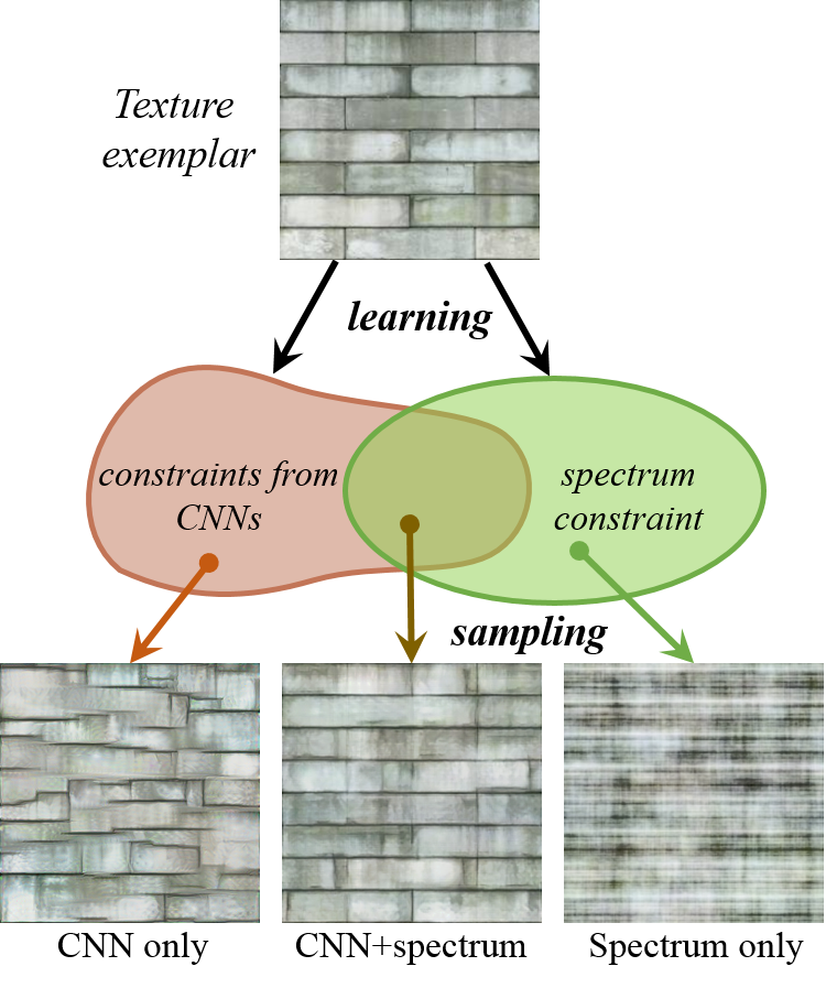
*Overview over their method, i.e. generated textures using style and/or spectrum-based loss.*
|
Precomputed Real-Time Texture Synthesis with Markovian Generative Adversarial Networks
Li, Chuan and Wand, Michael
European Conference on Computer Vision - 2016 via Local Bibsonomy
Keywords: dblp
Li, Chuan and Wand, Michael
European Conference on Computer Vision - 2016 via Local Bibsonomy
Keywords: dblp
|
[link]
https://www.youtube.com/watch?v=PRD8LpPvdHI
* They describe a method that can be used for two problems:
* (1) Choose a style image and apply that style to other images.
* (2) Choose an example texture image and create new texture images that look similar.
* In contrast to previous methods their method can be applied very fast to images (style transfer) or noise (texture creation). However, per style/texture a single (expensive) initial training session is still necessary.
* Their method builds upon their previous paper "Combining Markov Random Fields and Convolutional Neural Networks for Image Synthesis".
### How
* Rough overview of their previous method:
* Transfer styles using three losses:
* Content loss: MSE between VGG representations.
* Regularization loss: Sum of x-gradient and y-gradients (encouraging smooth areas).
* MRF-based style loss: Sample `k x k` patches from VGG representations of content image and style image. For each patch from content image find the nearest neighbor (based on normalized cross correlation) from style patches. Loss is then the sum of squared errors of euclidean distances between content patches and their nearest neighbors.
* Generation of new images is done by starting with noise and then iteratively applying changes that minimize the loss function.
* They introduce mostly two major changes:
* (a) Get rid of the costly nearest neighbor search for the MRF loss. Instead, use a discriminator-network that receives a patch and rates how real that patch looks.
* This discriminator-network is costly to train, but that only has to be done once (per style/texture).
* (b) Get rid of the slow, iterative generation of images. Instead, start with the content image (style transfer) or noise image (texture generation) and feed that through a single generator-network to create the output image (with transfered style or generated texture).
* This generator-network is costly to train, but that only has to be done once (per style/texture).
* MDANs
* They implement change (a) to the standard architecture and call that an "MDAN" (Markovian Deconvolutional Adversarial Networks).
* So the architecture of the MDAN is:
* Input: Image (RGB pixels)
* Branch 1: Markovian Patch Quality Rater (aka Discriminator)
* Starts by feeding the image through VGG19 until layer `relu3_1`. (Note: VGG weights are fixed/not trained.)
* Then extracts `k x k` patches from the generated representations.
* Feeds each patch through a shallow ConvNet (convolution with BN then fully connected layer).
* Training loss is a hinge loss, i.e. max margin between classes +1 (real looking patch) and -1 (fake looking patch). (Could also take a single sigmoid output, but they argue that hinge loss isn't as likely to saturate.)
* This branch will be trained continuously while synthesizing a new image.
* Branch 2: Content Estimation/Guidance
* Note: This branch is only used for style transfer, i.e if using an content image and not for texture generation.
* Starts by feeding the currently synthesized image through VGG19 until layer `relu5_1`. (Note: VGG weights are fixed/not trained.)
* Also feeds the content image through VGG19 until layer `relu5_1`.
* Then uses a MSE loss between both representations (so similar to a MSE on RGB pixels that is often used in autoencoders).
* Nothing in this branch needs to trained, the loss only affects the synthesizing of the image.
* MGANs
* The MGAN is like the MDAN, but additionally implements change (b), i.e. they add a generator that takes an image and stylizes it.
* The generator's architecture is:
* Input: Image (RGB pixels) or noise (for texture synthesis)
* Output: Image (RGB pixels) (stylized input image or generated texture)
* The generator takes the image (pixels) and feeds that through VGG19 until layer `relu4_1`.
* Similar to the DCGAN generator, they then apply a few fractionally strided convolutions (with BN and LeakyReLUs) to that, ending in a Tanh output. (Fractionally strided convolutions increase the height/width of the images, here to compensate the VGG pooling layers.)
* The output after the Tanh is the output image (RGB pixels).
* They train the generator with pairs of `(input image, stylized image or texture)`. These pairs can be gathered by first running the MDAN alone on several images. (With significant augmentation a few dozen pairs already seem to be enough.)
* One of two possible loss functions can then be used:
* Simple standard choice: MSE on the euclidean distance between expected output pixels and generated output pixels. Can cause blurriness.
* Better choice: MSE on a higher VGG representation. Simply feed the generated output pixels through VGG19 until `relu4_1` and the reuse the already generated (see above) VGG-representation of the input image. This is very similar to the pixel-wise comparison, but tends to cause less blurriness.
* Note: For some reason the authors call their generator a VAE, but don't mention any typical VAE technique, so it's not described like one here.
* They use Adam to train their networks.
* For texture generation they use Perlin Noise instead of simple white noise. In Perlin Noise, lower frequency components dominate more than higher frequency components. White noise didn't work well with the VGG representations in the generator (activations were close to zero).
### Results
* Similar quality like previous methods, but much faster (compared to most methods).
* For the Markovian Patch Quality Rater (MDAN branch 1):
* They found that the weights of this branch can be used as initialization for other training sessions (e.g. other texture styles), leading to a decrease in required iterations/epochs.
* Using VGG for feature extraction seems to be crucial. Training from scratch generated in worse results.
* Using larger patch sizes preserves more structure of the structure of the style image/texture. Smaller patches leads to more flexibility in generated patterns.
* They found that using more than 3 convolutional layers or more than 64 filters per layer provided no visible benefit in quality.

*Result of their method, compared to other methods.*

*Architecture of their model.*
|
Semantic Style Transfer and Turning Two-Bit Doodles into Fine Artworks
Alex J. Champandard
arXiv e-Print archive - 2016 via Local arXiv
Keywords: cs.CV
First published: 2016/03/05 (8 years ago)
Abstract: Convolutional neural networks (CNNs) have proven highly effective at image synthesis and style transfer. For most users, however, using them as tools can be a challenging task due to their unpredictable behavior that goes against common intuitions. This paper introduces a novel concept to augment such generative architectures with semantic annotations, either by manually authoring pixel labels or using existing solutions for semantic segmentation. The result is a content-aware generative algorithm that offers meaningful control over the outcome. Thus, we increase the quality of images generated by avoiding common glitches, make the results look significantly more plausible, and extend the functional range of these algorithms---whether for portraits or landscapes, etc. Applications include semantic style transfer and turning doodles with few colors into masterful paintings!
more
less
Alex J. Champandard
arXiv e-Print archive - 2016 via Local arXiv
Keywords: cs.CV
First published: 2016/03/05 (8 years ago)
Abstract: Convolutional neural networks (CNNs) have proven highly effective at image synthesis and style transfer. For most users, however, using them as tools can be a challenging task due to their unpredictable behavior that goes against common intuitions. This paper introduces a novel concept to augment such generative architectures with semantic annotations, either by manually authoring pixel labels or using existing solutions for semantic segmentation. The result is a content-aware generative algorithm that offers meaningful control over the outcome. Thus, we increase the quality of images generated by avoiding common glitches, make the results look significantly more plausible, and extend the functional range of these algorithms---whether for portraits or landscapes, etc. Applications include semantic style transfer and turning doodles with few colors into masterful paintings!
|
[link]
* They describe a method to transfer image styles based on semantic classes.
* This allows to:
* (1) Transfer styles between images more accurately than with previous models. E.g. so that the background of an image does not receive the style of skin/hair/clothes/... seen in the style image. Skin in the synthesized image should receive the style of skin from the style image. Same for hair, clothes, etc.
* (2) Turn simple doodles into artwork by treating the simplified areas in the doodle as semantic classes and annotating an artwork with these same semantic classes. (E.g. "this blob should receive the style from these trees.")
### How
* Their method is based on [Combining Markov Random Fields and Convolutional Neural Networks for Image Synthesis](Combining_MRFs_and_CNNs_for_Image_Synthesis.md).
* They use the same content loss and mostly the same MRF-based style loss. (Apparently they don't use the regularization loss.)
* They change the input of the MRF-based style loss.
* Usually that input would only be the activations of a VGG-layer (for the synthesized image or the style source image).
* They add a semantic map with weighting `gamma` to the activation, i.e. `<representation of image> = <activation of specific layer for that image> || gamma * <semantic map>`.
* The semantic map has N channels with 1s in a channel where a specific class is located (e.g. skin).
* The semantic map has to be created by the user for both the content image and the style image.
* As usually for the MRF loss, patches are then sampled from the representations. The semantic maps then influence the distance measure. I.e. patches are more likely to be sampled from the same semantic class.
* Higher `gamma` values make it more likely to sample from the same semantic class (because the distance from patches from different classes gets larger).
* One can create a small doodle with few colors, then use the colors as the semantic map. Then add a semantic map to an artwork and run the algorithm to transform the doodle into an artwork.
### Results
* More control over the transfered styles than previously.
* Less sensitive to the style weighting, because of the additional `gamma` hyperparameter.
* Easy transformation from doodle to artwork.

*Turning a doodle into an artwork. Note that the doodle input image is also used as the semantic map of the input.*
|
Combining Markov Random Fields and Convolutional Neural Networks for Image Synthesis
Li, Chuan and Wand, Michael
Conference and Computer Vision and Pattern Recognition - 2016 via Local Bibsonomy
Keywords: dblp
Li, Chuan and Wand, Michael
Conference and Computer Vision and Pattern Recognition - 2016 via Local Bibsonomy
Keywords: dblp
|
[link]
* They describe a method that applies the style of a source image to a target image.
* Example: Let a normal photo look like a van Gogh painting.
* Example: Let a normal car look more like a specific luxury car.
* Their method builds upon the well known artistic style paper and uses a new MRF prior.
* The prior leads to locally more plausible patterns (e.g. less artifacts).
### How
* They reuse the content loss from the artistic style paper.
* The content loss was calculated by feed the source and target image through a network (here: VGG19) and then estimating the squared error of the euclidean distance between one or more hidden layer activations.
* They use layer `relu4_2` for the distance measurement.
* They replace the original style loss with a MRF based style loss.
* Step 1: Extract from the source image `k x k` sized overlapping patches.
* Step 2: Perform step (1) analogously for the target image.
* Step 3: Feed the source image patches through a pretrained network (here: VGG19) and select the representations `r_s` from specific hidden layers (here: `relu3_1`, `relu4_1`).
* Step 4: Perform step (3) analogously for the target image. (Result: `r_t`)
* Step 5: For each patch of `r_s` find the best matching patch in `r_t` (based on normalized cross correlation).
* Step 6: Calculate the sum of squared errors (based on euclidean distances) of each patch in `r_s` and its best match (according to step 5).
* They add a regularizer loss.
* The loss encourages smooth transitions in the synthesized image (i.e. few edges, corners).
* It is based on the raw pixel values of the last synthesized image.
* For each pixel in the synthesized image, they calculate the squared x-gradient and the squared y-gradient and then add both.
* They use the sum of all those values as their loss (i.e. `regularizer loss = <sum over all pixels> x-gradient^2 + y-gradient^2`).
* Their whole optimization problem is then roughly `image = argmin_image MRF-style-loss + alpha1 * content-loss + alpha2 * regularizer-loss`.
* In practice, they start their synthesis with a low resolution image and then progressively increase the resolution (each time performing some iterations of optimization).
* In practice, they sample patches from the style image under several different rotations and scalings.
### Results
* In comparison to the original artistic style paper:
* Less artifacts.
* Their method tends to preserve style better, but content worse.
* Can handle photorealistic style transfer better, so long as the images are similar enough. If no good matches between patches can be found, their method performs worse.
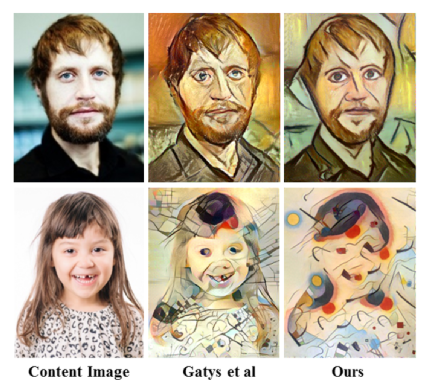
*Non-photorealistic example images. Their method vs. the one from the original artistic style paper.*
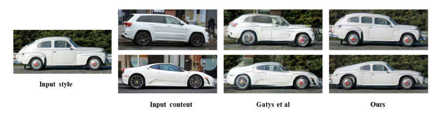
*Photorealistic example images. Their method vs. the one from the original artistic style paper.*
|
Accurate Image Super-Resolution Using Very Deep Convolutional Networks
Kim, Jiwon and Lee, Jung Kwon and Lee, Kyoung Mu
Conference and Computer Vision and Pattern Recognition - 2016 via Local Bibsonomy
Keywords: dblp
Kim, Jiwon and Lee, Jung Kwon and Lee, Kyoung Mu
Conference and Computer Vision and Pattern Recognition - 2016 via Local Bibsonomy
Keywords: dblp
|
[link]
* They describe a model that upscales low resolution images to their high resolution equivalents ("Single Image Super Resolution").
* Their model uses a deeper architecture than previous models and has a residual component.
### How
* Their model is a fully convolutional neural network.
* Input of the model: The image to upscale, *already upscaled to the desired size* (but still blurry).
* Output of the model: The upscaled image (without the blurriness).
* They use 20 layers of padded 3x3 convolutions with size 64xHxW with ReLU activations. (No pooling.)
* They have a residual component, i.e. the model only learns and outputs the *change* that has to be applied/added to the blurry input image (instead of outputting the full image). That change is applied to the blurry input image before using the loss function on it. (Note that this is a bit different from the currently used "residual learning".)
* They use a MSE between the "correct" upscaling and the generated upscaled image (input image + residual).
* They use SGD starting with a learning rate of 0.1 and decay it 3 times by a factor of 10.
* They use weight decay of 0.0001.
* During training they use a special gradient clipping adapted to the learning rate. Usually gradient clipping restricts the gradient values to `[-t, t]` (`t` is a hyperparameter). Their gradient clipping restricts the values to `[-t/lr, t/lr]` (where `lr` is the learning rate).
* They argue that their special gradient clipping allows the use of significantly higher learning rates.
* They train their model on multiple scales, e.g. 2x, 3x, 4x upscaling. (Not really clear how. They probably feed their upscaled image again into the network or something like that?)
### Results
* Higher accuracy upscaling than all previous methods.
* Can handle well upscaling factors above 2x.
* Residual network learns significantly faster than non-residual network.

*Architecture of the model.*

*Super-resolution quality of their model (top, bottom is a competing model).*
|
Hierarchical Deep Reinforcement Learning: Integrating Temporal Abstraction and Intrinsic Motivation
Tejas D. Kulkarni and Karthik R. Narasimhan and Ardavan Saeedi and Joshua B. Tenenbaum
arXiv e-Print archive - 2016 via Local arXiv
Keywords: cs.LG, cs.AI, cs.CV, cs.NE, stat.ML
First published: 2016/04/20 (8 years ago)
Abstract: Learning goal-directed behavior in environments with sparse feedback is a major challenge for reinforcement learning algorithms. The primary difficulty arises due to insufficient exploration, resulting in an agent being unable to learn robust value functions. Intrinsically motivated agents can explore new behavior for its own sake rather than to directly solve problems. Such intrinsic behaviors could eventually help the agent solve tasks posed by the environment. We present hierarchical-DQN (h-DQN), a framework to integrate hierarchical value functions, operating at different temporal scales, with intrinsically motivated deep reinforcement learning. A top-level value function learns a policy over intrinsic goals, and a lower-level function learns a policy over atomic actions to satisfy the given goals. h-DQN allows for flexible goal specifications, such as functions over entities and relations. This provides an efficient space for exploration in complicated environments. We demonstrate the strength of our approach on two problems with very sparse, delayed feedback: (1) a complex discrete stochastic decision process, and (2) the classic ATARI game `Montezuma's Revenge'.
more
less
Tejas D. Kulkarni and Karthik R. Narasimhan and Ardavan Saeedi and Joshua B. Tenenbaum
arXiv e-Print archive - 2016 via Local arXiv
Keywords: cs.LG, cs.AI, cs.CV, cs.NE, stat.ML
First published: 2016/04/20 (8 years ago)
Abstract: Learning goal-directed behavior in environments with sparse feedback is a major challenge for reinforcement learning algorithms. The primary difficulty arises due to insufficient exploration, resulting in an agent being unable to learn robust value functions. Intrinsically motivated agents can explore new behavior for its own sake rather than to directly solve problems. Such intrinsic behaviors could eventually help the agent solve tasks posed by the environment. We present hierarchical-DQN (h-DQN), a framework to integrate hierarchical value functions, operating at different temporal scales, with intrinsically motivated deep reinforcement learning. A top-level value function learns a policy over intrinsic goals, and a lower-level function learns a policy over atomic actions to satisfy the given goals. h-DQN allows for flexible goal specifications, such as functions over entities and relations. This provides an efficient space for exploration in complicated environments. We demonstrate the strength of our approach on two problems with very sparse, delayed feedback: (1) a complex discrete stochastic decision process, and (2) the classic ATARI game `Montezuma's Revenge'.
|
[link]
  * They present a hierarchical method for reinforcement learning.
  * The method combines "long"-term goals with short-term action choices.

### How
  * They have two components:
    * Meta-Controller:
      * Responsible for the "long"-term goals.
      * Is trained to pick goals (based on the current state) that maximize (extrinsic) rewards, just like you would usually optimize to maximize rewards by picking good actions.
      * The Meta-Controller only picks goals when the Controller terminates or achieved the goal.
    * Controller:
      * Receives the current state and the current goal.
      * Has to pick a reward maximizing action based on those, just as the agent would usually do (only the goal is added here).
      * The reward is intrinsic. It comes from the Critic. The Critic gives reward whenever the current goal is reached.
  * For Montezuma's Revenge:
    * A goal is to reach a specific object.
    * The goal is encoded via a bitmask (as big as the game screen). The mask contains 1s wherever the object is.
    * They hand-extract the location of a few specific objects.
    * So basically:
      * The Meta-Controller picks the next object to reach via a Q-value function.
      * It receives extrinsic reward when objects have been reached in a specific sequence.
      * The Controller picks actions that lead to reaching the object based on a Q-value function. It iterates action-choosing until it terminates or reached the goal-object.
      * The Critic awards intrinsic reward to the Controller whenever the goal-object was reached.
    * They use CNNs for the Meta-Controller and the Controller, similar in architecture to the Atari-DQN paper (shallow CNNs).
    * They use two replay memories, one for the Meta-Controller (size 40k) and one for the Controller (size 1M).
    * Both follow an epsilon-greedy policy (for picking goals/actions). Epsilon starts at 1.0 and is annealed down to 0.1.
    * They use a discount factor / gamma of 0.9.
    * They train with SGD.

### Results
  * Learns to play Montezuma's Revenge.
  * Learns to act well in a more abstract MDP with delayed rewards and where simple Q-learning failed.

--------------------

# Rough chapter-wise notes


* (1) Introduction
  * Basic problem: Learn goal directed behaviour from sparse feedbacks.
  * Challenges:
    * Explore state space efficiently
    * Create multiple levels of spatio-temporal abstractions
  * Their method: Combines deep reinforcement learning with hierarchical value functions.
  * Their agent is motivated to solve specific intrinsic goals.
  * Goals are defined in the space of entities and relations, which constraints the search space.
  * They define their value function as V(s, g) where s is the state and g is a goal.
  * First, their agent learns to solve intrinsically generated goals. Then it learns to chain these goals together.
  * Their model has two hiearchy levels:
    * Meta-Controller: Selects the current goal based on the current state.
    * Controller: Takes state s and goal g, then selects a good action based on s and g. The controller operates until g is achieved, then the meta-controller picks the next goal.
  * Meta-Controller gets extrinsic rewards, controller gets intrinsic rewards.
  * They use SGD to optimize the whole system (with respect to reward maximization).

* (3) Model
  * Basic setting: Action a out of all actions A, state s out of S, transition function T(s,a)->s', reward by state F(s)->R.
  * epsilon-greedy is good for local exploration, but it's not good at exploring very different areas of the state space.
  * They use intrinsically motivated goals to better explore the state space.
  * Sequences of goals are arranged to maximize the received extrinsic reward.
  * The agent learns one policy per goal.
  * Meta-Controller: Receives current state, chooses goal.
  * Controller: Receives current state and current goal, chooses action. Keeps choosing actions until goal is achieved or a terminal state is reached. Has the optimization target of maximizing cumulative reward.
  * Critic: Checks if current goal is achieved and if so provides intrinsic reward.
  * They use deep Q learning to train their model.
  * There are two Q-value functions. One for the controller and one for the meta-controller.
  * Both formulas are extended by the last chosen goal g.
  * The Q-value function of the meta-controller does not depend on the chosen action.
  * The Q-value function of the controller receives only intrinsic direct reward, not extrinsic direct reward.
  * Both Q-value functions are reprsented with DQNs.
  * Both are optimized to minimize MSE losses.
  * They use separate replay memories for the controller and meta-controller.
  * A memory is added for the meta-controller whenever the controller terminates.
  * Each new goal is picked by the meta-controller epsilon-greedy (based on the current state).
  * The controller picks actions epsilon-greedy (based on the current state and goal).
  * Both epsilons are annealed down.

* (4) Experiments
  * (4.1) Discrete MDP with delayed rewards
    * Basic MDP setting, following roughly: Several states (s1 to s6) organized in a chain. The agent can move left or right. It gets high reward if it moves to state s6 and then back to s1, otherwise it gets small reward per reached state.
    * They use their hierarchical method, but without neural nets.
    * Baseline is Q-learning without a hierarchy/intrinsic rewards.
    * Their method performs significantly better than the baseline.
  * (4.2) ATARI game with delayed rewards
    * They play Montezuma's Revenge with their method, because that game has very delayed rewards.
    * They use CNNs for the controller and meta-controller (architecture similar to the Atari-DQN paper).
    * The critic reacts to (entity1, relation, entity2) relationships. The entities are just objects visible in the game. The relation is (apparently ?) always "reached", i.e. whether object1 arrived at object2.
    * They extract the objects manually, i.e. assume the existance of a perfect unsupervised object detector.
    * They encode the goals apparently not as vectors, but instead just use a bitmask (game screen heightand width), which has 1s at the pixels that show the object.
    * Replay memory sizes: 1M for controller, 50k for meta-controller.
    * gamma=0.99
    * They first only train the controller (i.e. meta-controller completely random) and only then train both jointly.
    * Their method successfully learns to perform actions which lead to rewards with long delays.
    * It starts with easier goals and then learns harder goals.
|
Artistic style transfer for videos
Manuel Ruder and Alexey Dosovitskiy and Thomas Brox
arXiv e-Print archive - 2016 via Local arXiv
Keywords: cs.CV
First published: 2016/04/28 (8 years ago)
Abstract: In the past, manually re-drawing an image in a certain artistic style required a professional artist and a long time. Doing this for a video sequence single-handed was beyond imagination. Nowadays computers provide new possibilities. We present an approach that transfers the style from one image (for example, a painting) to a whole video sequence. We make use of recent advances in style transfer in still images and propose new initializations and loss functions applicable to videos. This allows us to generate consistent and stable stylized video sequences, even in cases with large motion and strong occlusion. We show that the proposed method clearly outperforms simpler baselines both qualitatively and quantitatively.
more
less
Manuel Ruder and Alexey Dosovitskiy and Thomas Brox
arXiv e-Print archive - 2016 via Local arXiv
Keywords: cs.CV
First published: 2016/04/28 (8 years ago)
Abstract: In the past, manually re-drawing an image in a certain artistic style required a professional artist and a long time. Doing this for a video sequence single-handed was beyond imagination. Nowadays computers provide new possibilities. We present an approach that transfers the style from one image (for example, a painting) to a whole video sequence. We make use of recent advances in style transfer in still images and propose new initializations and loss functions applicable to videos. This allows us to generate consistent and stable stylized video sequences, even in cases with large motion and strong occlusion. We show that the proposed method clearly outperforms simpler baselines both qualitatively and quantitatively.
|
[link]
https://www.youtube.com/watch?v=vQk_Sfl7kSc&feature=youtu.be

  * The paper describes a method to transfer the style (e.g. choice of colors, structure of brush strokes) of an image to a whole video.
  * The method is designed so that the transfered style is consistent over many frames.
  * Examples for such consistency:
    * No flickering of style between frames. So the next frame has always roughly the same style in the same locations.
    * No artefacts at the boundaries of objects, even if they are moving.
    * If an area gets occluded and then unoccluded a few frames later, the style of that area is still the same as before the occlusion.

### How
  * Assume that we have a frame to stylize $x$ and an image from which to extract the style $a$.
  * The basic process is the same as in the original Artistic Style Transfer paper, they just add a bit on top of that.
  * They start with a gaussian noise image $x'$ and change it gradually so that a loss function gets minimized.
  * The loss function has the following components:
    * Content loss *(old, same as in the Artistic Style Transfer paper)*
      * This loss makes sure that the content in the generated/stylized image still matches the content of the original image.
      * $x$ and $x'$ are fed forward through a pretrained network (VGG in their case).
      * Then the generated representations of the intermediate layers of the network are extracted/read.
      * One or more layers are picked and the difference between those layers for $x$ and $x'$ is measured via a MSE.
      * E.g. if we used only the representations of the layer conv5 then we would get something like `(conv5(x) - conv5(x'))^2` per example. (Where conv5() also executes all previous layers.)
    * Style loss *(old)*
      * This loss makes sure that the style of the generated/stylized image matches the style source $a$.
      * $x'$ and $a$ are fed forward through a pretrained network (VGG in their case).
      * Then the generated representations of the intermediate layers of the network are extracted/read.
      * One or more layers are picked and the Gram Matrices of those layers are calculated.
      * Then the difference between those matrices is measured via a MSE.
    * Temporal loss *(new)*
      * This loss enforces consistency in style between a pair of frames.
      * The main sources of inconsistency are boundaries of moving objects and areas that get unonccluded.
      * They use the optical flow to detect motion.
        * Applying an optical flow method to two frames $(i, i+1)$ returns per pixel the movement of that pixel, i.e. if the pixel at $(x=1, y=2)$ moved to $(x=2, y=4)$ the optical flow at that pixel would be $(u=1, v=2)$.
        * The optical flow can be split into the forward flow (here `fw`) and the backward flow (here `bw`). The forward flow is the flow from frame i to i+1 (as described in the previous point). The backward flow is the flow from frame $i+1$ to $i$ (reverse direction in time).
      * Boundaries
        * At boundaries of objects the derivative of the flow is high, i.e. the flow "suddenly" changes significantly from one pixel to the other.
        * So to detect boundaries they use (per pixel) roughly the equation `gradient(u)^2 + gradient(v)^2 > length((u,v))`.
      * Occlusions and disocclusions
        * If a pixel does not get occluded/disoccluded between frames, the optical flow method should be able to correctly estimate the motion of that pixel between the frames. The forward and backward flows then should be roughly equal, just in opposing directions.
        * If a pixel does get occluded/disoccluded between frames, it will not be visible in one the two frames and therefore the optical flow method cannot reliably estimate the motion for that pixel. It is then expected that the forward and backward flow are unequal.
        * To measure that effect they roughly use (per pixel) a formula matching `length(fw + bw)^2 > length(fw)^2 + length(bw)^2`.
      * Mask $c$
        * They create a mask $c$ with the size of the frame.
        * For every pixel they estimate whether the boundary-equation *or* the disocclusion-equation is true.
        * If either of them is true, they add a 0 to the mask, otherwise a 1. So the mask is 1 wherever there is *no* disocclusion or motion boundary.
      * Combination
        * The final temporal loss is the mean (over all pixels) of $c*(x-w)^2$.
          * $x$ is the frame to stylize.
          * $w$ is the previous *stylized* frame (frame i-1), warped according to the optical flow between frame i-1 and i.
          * `c` is the mask value at the pixel.
        * By using the difference `x-w` they ensure that the difference in styles between two frames is low.
        * By adding `c` they ensure the style-consistency only at pixels that probably should have a consistent style.
    * Long-term loss *(new)*
      * This loss enforces consistency in style between pairs of frames that are longer apart from each other.
      * It is a simple extension of the temporal (short-term) loss.
      * The temporal loss was computed for frames (i-1, i). The long-term loss is the sum of the temporal losses for the frame pairs {(i-4,i), (i-2,i), (i-1,i)}.
      * The $c$ mask is recomputed for every pair and 1 if there are no boundaries/disocclusions detected, but only if there is not a 1 for the same pixel in a later mask. The additional condition is intended to associate pixels with their closest neighbours in time to minimize possible errors.
      * Note that the long-term loss can completely replace the temporal loss as the latter one is contained in the former one.
  * Multi-pass approach *(new)*
    * They had problems with contrast around the boundaries of the frames.
    * To combat that, they use a multi-pass method in which they seem to calculate the optical flow in multiple forward and backward passes? (Not very clear here what they do and why it would help.)
  * Initialization with previous frame *(new)*
    * Instead of starting at a gaussian noise image every time, they instead use the previous stylized frame.
    * That immediately leads to more similarity between the frames.
|
Noisy Activation Functions
Gülçehre, Çaglar and Moczulski, Marcin and Denil, Misha and Bengio, Yoshua
International Conference on Machine Learning - 2016 via Local Bibsonomy
Keywords: dblp
Gülçehre, Çaglar and Moczulski, Marcin and Denil, Misha and Bengio, Yoshua
International Conference on Machine Learning - 2016 via Local Bibsonomy
Keywords: dblp
|
[link]
* Certain activation functions, mainly sigmoid, tanh, hard-sigmoid and hard-tanh can saturate.
* That means that their gradient is either flat 0 after threshold values (e.g. -1 and +1) or that it approaches zero for high/low values.
* If there's no gradient, training becomes slow or stops completely.
* That's a problem, because sigmoid, tanh, hard-sigmoid and hard-tanh are still often used in some models, like LSTMs, GRUs or Neural Turing Machines.
* To fix the saturation problem, they add noise to the output of the activation functions.
* The noise increases as the unit saturates.
* Intuitively, once the unit is saturating, it will occasionally "test" an activation in the non-saturating regime to see if that output performs better.
### How
* The basic formula is: `phi(x,z) = alpha*h(x) + (1-alpha)u(x) + d(x)std(x)epsilon`
* Variables in that formula:
* Non-linear part `alpha*h(x)`:
* `alpha`: A constant hyperparameter that determines the "direction" of the noise and the slope. Values below 1.0 let the noise point away from the unsaturated regime. Values <=1.0 let it point towards the unsaturated regime (higher alpha = stronger noise).
* `h(x)`: The original activation function.
* Linear part `(1-alpha)u(x)`:
* `u(x)`: First-order Taylor expansion of h(x).
* For sigmoid: `u(x) = 0.25x + 0.5`
* For tanh: `u(x) = x`
* For hard-sigmoid: `u(x) = max(min(0.25x+0.5, 1), 0)`
* For hard-tanh: `u(x) = max(min(x, 1), -1)`
* Noise/Stochastic part `d(x)std(x)epsilon`:
* `d(x) = -sgn(x)sgn(1-alpha)`: Changes the "direction" of the noise.
* `std(x) = c(sigmoid(p*v(x))-0.5)^2 = c(sigmoid(p*(h(x)-u(x)))-0.5)^2`
* `c` is a hyperparameter that controls the scale of the standard deviation of the noise.
* `p` controls the magnitude of the noise. Due to the `sigmoid(y)-0.5` this can influence the sign. `p` is learned.
* `epsilon`: A noise creating random variable. Usually either a Gaussian or the positive half of a Gaussian (i.e. `z` or `|z|`).
* The hyperparameter `c` can be initialized at a high value and then gradually decreased over time. That would be comparable to simulated annealing.
* Noise could also be applied to the input, i.e. `h(x)` becomes `h(x + noise)`.
### Results
* They replaced sigmoid/tanh/hard-sigmoid/hard-tanh units in various experiments (without further optimizations).
* The experiments were:
* Learn to execute source code (LSTM?)
* Language model from Penntreebank (2-layer LSTM)
* Neural Machine Translation engine trained on Europarl (LSTM?)
* Image caption generation with soft attention trained on Flickr8k (LSTM)
* Counting unique integers in a sequence of integers (LSTM)
* Associative recall (Neural Turing Machine)
* Noisy activations practically always led to a small or moderate improvement in resulting accuracy/NLL/BLEU.
* In one experiment annealed noise significantly outperformed unannealed noise, even beating careful curriculum learning. (Somehow there are not more experiments about that.)
* The Neural Turing Machine learned far faster with noisy activations and also converged to a much better solution.

*Hard-tanh with noise for various alphas. Noise increases in different ways in the saturing regimes.*

*Performance during training of a Neural Turing Machine with and without noisy activation units.*
--------------------
# Rough chapter-wise notes
* (1) Introduction
* ReLU and Maxout activation functions have improved the capabilities of training deep networks.
* Previously, tanh and sigmoid were used, which were only suited for shallow networks, because they saturate, which kills the gradient.
* They suggest a different avenue: Use saturating nonlinearities, but inject noise when they start to saturate (and let the network learn how much noise is "good").
* The noise allows to train deep networks with saturating activation functions.
* Many current architectures (LSTMs, GRUs, Neural Turing Machines, ...) require "hard" decisions (yes/no). But they use "soft" activation functions to implement those, because hard functions lack gradient.
* The soft activation functions can still saturate (no more gradient) and don't match the nature of the binary decision problem. So it would be good to replace them with something better.
* They instead use hard activation functions and compensate for the lack of gradient by using noise (during training).
* Networks with hard activation functions outperform those with soft ones.
* (2) Saturating Activation Functions
* Activation Function = A function that maps a real value to a new real value and is differentiable almost everywhere.
* Right saturation = The gradient of an activation function becomes 0 if the input value goes towards infinity.
* Left saturation = The gradient of an activation function becomes 0 if the input value goes towards -infinity.
* Saturation = A activation function saturates if it right-saturates and left-saturates.
* Hard saturation = If there is a constant c for which for which the gradient becomes 0.
* Soft saturation = If there is no constant, i.e. the input value must become +/- infinity.
* Soft saturating activation functions can be converted to hard saturating ones by using a first-order Taylor expansion and then clipping the values to the required range (e.g. 0 to 1).
* A hard activating tanh is just `f(x) = x`. With clipping to [-1, 1]: `max(min(f(x), 1), -1)`.
* The gradient for hard activation functions is 0 above/below certain constants, which will make training significantly more challenging.
* hard-sigmoid, sigmoid and tanh are contractive mappings, hard-tanh for some reason only when it's greater than the threshold.
* The fixed-point for tanh is 0, for the others !=0. That can have influences on the training performance.
* (3) Annealing with Noisy Activation Functions
* Suppose that there is an activation function like hard-sigmoid or hard-tanh with additional noise (iid, mean=0, variance=std^2).
* If the noise's `std` is 0 then the activation function is the original, deterministic one.
* If the noise's `std` is very high then the derivatives and gradient become high too. The noise then "drowns" signal and the optimizer just moves randomly through the parameter space.
* Let the signal to noise ratio be `SNR = std_signal / std_noise`. So if SNR is low then noise drowns the signal and exploration is random.
* By letting SNR grow (i.e. decreaseing `std_noise`) we switch the model to fine tuning mode (less coarse exploration).
* That is similar to simulated annealing, where noise is also gradually decreased to focus on better and better regions of the parameter space.
* (4) Adding Noise when the Unit Saturate
* This approach does not always add the same noise. Instead, noise is added proportinally to the saturation magnitude. More saturation, more noise.
* That results in a clean signal in "good" regimes (non-saturation, strong gradients) and a noisy signal in "bad" regimes (saturation).
* Basic activation function with noise: `phi(x, z) = h(x) + (mu + std(x)*z)`, where `h(x)` is the saturating activation function, `mu` is the mean of the noise, `std` is the standard deviation of the noise and `z` is a random variable.
* Ideally the noise is unbiased so that the expectation values of `phi(x,z)` and `h(x)` are the same.
* `std(x)` should take higher values as h(x) enters the saturating regime.
* To calculate how "saturating" a activation function is, one can `v(x) = h(x) - u(x)`, where `u(x)` is the first-order Taylor expansion of `h(x)`.
* Empirically they found that a good choice is `std(x) = c(sigmoid(p*v(x)) - 0.5)^2` where `c` is a hyperparameter and `p` is learned.
* (4.1) Derivatives in the Saturated Regime
* For values below the threshold, the gradient of the noisy activation function is identical to the normal activation function.
* For values above the threshold, the gradient of the noisy activation function is `phi'(x,z) = std'(x)*z`. (Assuming that z is unbiased so that mu=0.)
* (4.2) Pushing Activations towards the Linear Regime
* In saturated regimes, one would like to have more of the noise point towards the unsaturated regimes than away from them (i.e. let the model try often whether the unsaturated regimes might be better).
* To achieve this they use the formula `phi(x,z) = alpha*h(x) + (1-alpha)u(x) + d(x)std(x)epsilon`
* `alpha`: A constant hyperparameter that determines the "direction" of the noise and the slope. Values below 1.0 let the noise point away from the unsaturated regime. Values <=1.0 let it point towards the unsaturated regime (higher alpha = stronger noise).
* `h(x)`: The original activation function.
* `u(x)`: First-order Taylor expansion of h(x).
* `d(x) = -sgn(x)sgn(1-alpha)`: Changes the "direction" of the noise.
* `std(x) = c(sigmoid(p*v(x))-0.5)^2 = c(sigmoid(p*(h(x)-u(x)))-0.5)^2` with `c` being a hyperparameter and `p` learned.
* `epsilon`: Either `z` or `|z|`. If `z` is a Gaussian, then `|z|` is called "half-normal" while just `z` is called "normal". Half-normal lets the noise only point towards one "direction" (towards the unsaturated regime or away from it), while normal noise lets it point in both directions (with the slope being influenced by `alpha`).
* The formula can be split into three parts:
* `alpha*h(x)`: Nonlinear part.
* `(1-alpha)u(x)`: Linear part.
* `d(x)std(x)epsilon`: Stochastic part.
* Each of these parts resembles a path along which gradient can flow through the network.
* During test time the activation function is made deterministic by using its expectation value: `E[phi(x,z)] = alpha*h(x) + (1-alpha)u(x) + d(x)std(x)E[epsilon]`.
* If `z` is half-normal then `E[epsilon] = sqrt(2/pi)`. If `z` is normal then `E[epsilon] = 0`.
* (5) Adding Noise to Input of the Function
* Noise can also be added to the input of an activation function, i.e. `h(x)` becomes `h(x + noise)`.
* The noise can either always be applied or only once the input passes a threshold.
* (6) Experimental Results
* They applied noise only during training.
* They used existing setups and just changed the activation functions to noisy ones. No further optimizations.
* `p` was initialized uniformly to [-1,1].
* Basic experiment settings:
* NAN: Normal noise applied to the outputs.
* NAH: Half-normal noise, i.e. `|z|`, i.e. noise is "directed" towards the unsaturated or satured regime.
* NANI: Normal noise applied to the *input*, i.e. `h(x+noise)`.
* NANIL: Normal noise applied to the input with learned variance.
* NANIS: Normal noise applied to the input, but only if the unit saturates (i.e. above/below thresholds).
* (6.1) Exploratory analysis
* A very simple MNIST network performed slightly better with noisy activations than without. But comparison was only to tanh and hard-tanh, not ReLU or similar.
* In an experiment with a simple GRU, NANI (noisy input) and NAN (noisy output) performed practically identical. NANIS (noisy input, only when saturated) performed significantly worse.
* (6.2) Learning to Execute
* Problem setting: Predict the output of some lines of code.
* They replaced sigmoids and tanhs with their noisy counterparts (NAH, i.e. half-normal noise on output). The model learned faster.
* (6.3) Penntreebank Experiments
* They trained a standard 2-layer LSTM language model on Penntreebank.
* Their model used noisy activations, as opposed to the usually non-noisy ones.
* They could improve upon the previously best value. Normal noise and half-normal noise performed roughly the same.
* (6.4) Neural Machine Translation Experiments
* They replaced all sigmoids and tanh units in the Neural Attention Model with noisy ones. Then they trained on the Europarl corpus.
* They improved upon the previously best score.
* (6.5) Image Caption Generation Experiments
* They train a network with soft attention to generate captions for the Flickr8k dataset.
* Using noisy activation units improved the result over normal sigmoids and tanhs.
* (6.6) Experiments with Continuation
* They build an LSTM and train it to predict how many unique integers there are in a sequence of random integers.
* Instead of using a constant value for hyperparameter `c` of the noisy activations (scale of the standard deviation of the noise), they start at `c=30` and anneal down to `c=0.5`.
* Annealed noise performed significantly better then unannealed noise.
* Noise applied to the output (NAN) significantly beat noise applied to the input (NANIL).
* In a second experiment they trained a Neural Turing Machine on the associative recall task.
* Again they used annealed noise.
* The NTM with annealed noise learned by far faster than the one without annealed noise and converged to a perfect solution.
|
Recurrent Neural Networks for Multivariate Time Series with Missing Values
Zhengping Che and Sanjay Purushotham and Kyunghyun Cho and David Sontag and Yan Liu
arXiv e-Print archive - 2016 via Local arXiv
Keywords: cs.LG, cs.NE, stat.ML
First published: 2016/06/06 (8 years ago)
Abstract: Many multivariate time series data in practical applications, such as health care, geoscience, and biology, are characterized by a variety of missing values. It has been noted that the missing patterns and values are often correlated with the target labels, a.k.a., missingness is informative, and there is significant interest to explore methods which model them for time series prediction and other related tasks. In this paper, we develop novel deep learning models based on Gated Recurrent Units (GRU), a state-of-the-art recurrent neural network, to handle missing observations. Our model takes two representations of missing patterns, i.e., masking and time duration, and effectively incorporates them into a deep model architecture so that it not only captures the long-term temporal dependencies in time series, but also utilizes the missing patterns to improve the prediction results. Experiments of time series classification tasks on real-world clinical datasets (MIMIC-III, PhysioNet) and synthetic datasets demonstrate that our models achieve state-of-art performance on these tasks and provide useful insights for time series with missing values.
more
less
Zhengping Che and Sanjay Purushotham and Kyunghyun Cho and David Sontag and Yan Liu
arXiv e-Print archive - 2016 via Local arXiv
Keywords: cs.LG, cs.NE, stat.ML
First published: 2016/06/06 (8 years ago)
Abstract: Many multivariate time series data in practical applications, such as health care, geoscience, and biology, are characterized by a variety of missing values. It has been noted that the missing patterns and values are often correlated with the target labels, a.k.a., missingness is informative, and there is significant interest to explore methods which model them for time series prediction and other related tasks. In this paper, we develop novel deep learning models based on Gated Recurrent Units (GRU), a state-of-the-art recurrent neural network, to handle missing observations. Our model takes two representations of missing patterns, i.e., masking and time duration, and effectively incorporates them into a deep model architecture so that it not only captures the long-term temporal dependencies in time series, but also utilizes the missing patterns to improve the prediction results. Experiments of time series classification tasks on real-world clinical datasets (MIMIC-III, PhysioNet) and synthetic datasets demonstrate that our models achieve state-of-art performance on these tasks and provide useful insights for time series with missing values.
|
[link]
#### Motivation:
+ When sampling a clinical time series, missing values become ubiquitous due to a variety of factors such as frequency of medical events (when a blood test is performed, for example).
+ Missing values can be very informative about the label - *informative missingness*.
+ The goal of the paper is to propose a deep learning model that **exploits the missingness patterns** to enhance its performance.
#### Time series notation:
Multivariate time series with $D$ variables of length $T$:
+ ${\bf X} = ({\bf x}_1, {\bf x}_2, \ldots, {\bf x}_T)^T \in \mathbb{R}^{T \times D}$.
+ ${\bf x}_t \in \mathbb{R}^{D}$ is the $t$-th measurement of all variables.
+ $x_t^d$ is the $d$-th component of ${\bf x}_t$.
Missing value information is incorporated using *masking* and *time-interval* concepts.
+ Masking: says which of the entries are missing values.
+ Masking vector ${\bf m}_t \in \{0, 1\}^D$, $m_t^d = 1$ if $x_t^d$ exists and $m_t^d = 0$ if $x_t^d$ is missing.
+ Time-interval: temporal pattern of 'no-missing' observations. Represented by time-stamps $s_t$ and time intervals $\delta_t$ (since its last observation).
Example:
${\bf X}$: input time series with 2 variables,
$$ {\bf X} = \begin{pmatrix}
47 & 49 & NA & 40 & NA & 43 & 55 \\ NA & 15 & 14 & NA & NA & NA & 15
\end{pmatrix}
$$
with time-stamps
$${\bf s} = \begin{pmatrix}
0 & 0.1 & 0.6 & 1.6 & 2.2 & 2.5 & 3.1
\end{pmatrix}
$$
The masking vectors ${\bf m}_t$ and time intervals ${\delta}_t$ for each variable are computed and stacked forming the masking matrix ${\bf M}$ and time interval matrix ${\bf \Delta}$ :
$$ {\bf M} = \begin{pmatrix}
1 & 1 & 0 & 1 & 0 & 1 & 1 \\ 0 & 1 & 1 & 0 & 0 & 0 & 1
\end{pmatrix}
$$
$$ {\bf \Delta} = \begin{pmatrix}
0 & 0.1 & 0.5 & 1.5 & 0.6 & 0.9 & 0.6 \\ 0 & 0.1 & 0.5 & 1.0 & 1.6 & 1.9 & 2.5
\end{pmatrix}
$$
#### Proposed Architecture:
+ GRU (Gated Recurrent Units) with "trainable" decays:
+ Input decay: which causes the variable to converge to its empirical mean instead of simply filling with the last value of the variable. The decay of each input is treated independently
+ Hidden state decay: Attempts to capture richer information from missing patterns. In this case the hidden state of the network at the previous time step is decayed.
#### Dataset:
+ MIMIC III v1.4: https://mimic.physionet.org/
+ Input events, Output events, Lab events, Prescription events
+ PhysioNet Challenge 2012: https://physionet.org/challenge/2012/
| MIMIC III | PhysioNet 2012 |
-----------------------------------|--------------|---------------------
Number of samples ($N$) | 19714 | 4000
Number of variables ($D$) |99 | 33
Mean number of time steps |35.89 | 68.91
Maximum number of time steps|150 | 155
Mean of variable missing rate |0.9621| 0.8225
#### Experiments and Results:
**Methodology**
+ Baselines:
+ Logistic Regression, SVM, Random Forest (PhysioNet sampled every 1h. MIMIC sampled every 2h). Forward / backfilling imputation. Masking vector is concatenated input to inform the models what inputs are imputed.
+ LSTM with mean imputation.
+ Variations of the proposed GRU model:
+ GRU-mean: impute average of the training set.
+ GRU-forward: impute last value.
+ GRU-simple: masking vectors and time interval are inputs. There is no imputation.
+ GRU-D: proposed model.
+ Batch normalization and dropout (p = 0.5) applied to the regression layer.
+ Normalized inputs to have a mean of 0 and standard deviation 1.
+ Parameter optimization: early stopping on validation set.
**Results**
Mortality Prediction (results in terms of AUC):
+ Proposed GRU-D outperforms other models on both datasets:
+ AUC = 0.8527 $\pm$ 0.003 for MIMIC-III and 0.8424 $\pm$ 0.012 for PhysioNet
+ Random Forest and SVM are the best non-RNN baselines.
+ GRU-simple was the best RNN variant.
Multitask Prediction (results in terms of AUC):
+ PhysioNet: mortality, <3 days, surgery, cardiac condition.
+ MIMIC III: 20 diagnostic categories.
+ The proposed GRU-D outperforms other baseline models.
#### Positive Aspects:
+ Instead of performing simple mean imputation or using indicator functions, the paper exploits missing values and missing patterns in a novel way.
+ The paper performs lengthy comparisons against baselines.
#### Caveats:
+ Clinical mortality datasets usually have very high imbalance between classes. In such cases, AUC alone is not the best metric to evaluate. It would have been interesting to see the results in terms of precision/recall.
|
End-to-End Deep Learning for Person Search
Tong Xiao and Shuang Li and Bochao Wang and Liang Lin and Xiaogang Wang
arXiv e-Print archive - 2016 via Local arXiv
Keywords: cs.CV
First published: 2016/04/07 (8 years ago)
Abstract: Existing person re-identification (re-id) benchmarks and algorithms mainly focus on matching cropped pedestrian images between queries and candidates. However, it is different from real-world scenarios where the annotations of pedestrian bounding boxes are unavailable and the target person needs to be found from whole images. To close the gap, we investigate how to localize and match query persons from the scene images without relying on the annotations of candidate boxes. Instead of breaking it down into two separate tasks---pedestrian detection and person re-id, we propose an end-to-end deep learning framework to jointly handle both tasks. A random sampling softmax loss is proposed to effectively train the model under the supervision of sparse and unbalanced labels. On the other hand, existing benchmarks are small in scale and the samples are collected from a few fixed camera views with low scene diversities. To address this issue, we collect a large-scale and scene-diversified person search dataset, which contains 18,184 images, 8,432 persons, and 99,809 annotated bounding boxes\footnote{\url{http://www.ee.cuhk.edu.hk/~xgwang/PS/dataset.html}}. We evaluate our approach and other baselines on the proposed dataset, and study the influence of various factors. Experiments show that our method achieves the best result.
more
less
Tong Xiao and Shuang Li and Bochao Wang and Liang Lin and Xiaogang Wang
arXiv e-Print archive - 2016 via Local arXiv
Keywords: cs.CV
First published: 2016/04/07 (8 years ago)
Abstract: Existing person re-identification (re-id) benchmarks and algorithms mainly focus on matching cropped pedestrian images between queries and candidates. However, it is different from real-world scenarios where the annotations of pedestrian bounding boxes are unavailable and the target person needs to be found from whole images. To close the gap, we investigate how to localize and match query persons from the scene images without relying on the annotations of candidate boxes. Instead of breaking it down into two separate tasks---pedestrian detection and person re-id, we propose an end-to-end deep learning framework to jointly handle both tasks. A random sampling softmax loss is proposed to effectively train the model under the supervision of sparse and unbalanced labels. On the other hand, existing benchmarks are small in scale and the samples are collected from a few fixed camera views with low scene diversities. To address this issue, we collect a large-scale and scene-diversified person search dataset, which contains 18,184 images, 8,432 persons, and 99,809 annotated bounding boxes\footnote{\url{http://www.ee.cuhk.edu.hk/~xgwang/PS/dataset.html}}. We evaluate our approach and other baselines on the proposed dataset, and study the influence of various factors. Experiments show that our method achieves the best result.
|
[link]
The paper presents a new deep learning framework for person search. The authors propose to unify two disjoint tasks of 'person detection' and 'person re-identification' into a single problem of 'person search' using a Convolutional Neural Network (CNN). Also, a new large-scale benchmark dataset for person search is collected and annotated. It contains $18,184$ images, $8,432$ identities, and $96,143$ pedestrian bounding boxes. Conventional person re-identification approaches detect people first and then extract features for each person, finally classifying to a category (as depicted in the figure below). Instead of breaking this into separate processes of detection and classification, the problem is solved jointly by using a single CNN similar to the Faster-RCNN framework. https://i.imgur.com/ISDQd9L.png The proposed framework (shown in the figure below) has a pedestrian proposal net which is used to detect people, and an identification net for extracting features for comparing with the target person. The two modules adapt with each other through joint optimization. In addition, a loss function called Online Instance Matching (OIM) is introduced to cope with problems of using Softmax or pairwise/triplet distance loss functions when the number of identities is large. A lookup table of features from all the labeled identities is maintained. In addition, the approach takes into account many unlabeled identities likely to appear in scene images, as negatives for labeled identities. There are no parameters to learn, the lookup table (LUT) and circular queue (CQ) are just feature buffers. When forward, each labeled identity is matched with all the stored features. When backward, the LUT is updated according to the ID, pushing new features to CQ, and pop out-of-date ones. https://i.imgur.com/1Smsi56.png To validate the approach, a new person search dataset is collected. On this dataset, the training accuracy when using Softmax loss is around $15\%$. However, with the OIM loss the accuracy improves consistently. Experiments are also performed to compare the method with baseline approaches. The baseline result is around $74\%$, while the proposed approach result (without unlabeled) is $76.1\%$ and $78.7\%$ with unlabeled data. |
Generating Images with Perceptual Similarity Metrics based on Deep Networks
Alexey Dosovitskiy and Thomas Brox
arXiv e-Print archive - 2016 via Local arXiv
Keywords: cs.LG, cs.CV, cs.NE
First published: 2016/02/08 (8 years ago)
Abstract: Image-generating machine learning models are typically trained with loss functions based on distance in the image space. This often leads to over-smoothed results. We propose a class of loss functions, which we call deep perceptual similarity metrics (DeePSiM), that mitigate this problem. Instead of computing distances in the image space, we compute distances between image features extracted by deep neural networks. This metric better reflects perceptually similarity of images and thus leads to better results. We show three applications: autoencoder training, a modification of a variational autoencoder, and inversion of deep convolutional networks. In all cases, the generated images look sharp and resemble natural images.
more
less
Alexey Dosovitskiy and Thomas Brox
arXiv e-Print archive - 2016 via Local arXiv
Keywords: cs.LG, cs.CV, cs.NE
First published: 2016/02/08 (8 years ago)
Abstract: Image-generating machine learning models are typically trained with loss functions based on distance in the image space. This often leads to over-smoothed results. We propose a class of loss functions, which we call deep perceptual similarity metrics (DeePSiM), that mitigate this problem. Instead of computing distances in the image space, we compute distances between image features extracted by deep neural networks. This metric better reflects perceptually similarity of images and thus leads to better results. We show three applications: autoencoder training, a modification of a variational autoencoder, and inversion of deep convolutional networks. In all cases, the generated images look sharp and resemble natural images.
|
[link]
This paper proposed a class of loss functions applicable to image generation that are based on distance in feature spaces:

$$\mathcal{L} = \lambda_{feat}\mathcal{L}_{feat} + \lambda_{adv}\mathcal{L}_{adv} + \lambda_{img}\mathcal{L}_{img}$$

### Key Points
- Using only l2 loss in image space yields over-smoothed results since it leads to averaging all likely locations of details.
- L_feat measures the distance in suitable feature space and therefore preserves distribution of fine details instead of exact locations.
- Using only L_feat yields bad results since feature representations are contractive. Many non-natural images also mapped to the same feature vector.
- By introducing a natural image prior - GAN, we can make sure that samples lie on the natural image manifold.

### Model

https://i.imgur.com/qNzMwQ6.png

### Exp
- Training Autoencoder
- Generate images using VAE
- Invert feature

### Thought
I think the experiment section is a little complicated to comprehend. However, the proposed loss seems really promising and can be applied to many tasks related to image generation.

### Questions
- Section 4.2 & 4.3 are hard to follow for me, need to pay more attention in the future
|

Synthesizing the preferred inputs for neurons in neural networks via deep generator networks
Nguyen, Anh and Dosovitskiy, Alexey and Yosinski, Jason and Brox, Thomas and Clune, Jeff
Neural Information Processing Systems Conference - 2016 via Local Bibsonomy
Keywords: dblp
Nguyen, Anh and Dosovitskiy, Alexey and Yosinski, Jason and Brox, Thomas and Clune, Jeff
Neural Information Processing Systems Conference - 2016 via Local Bibsonomy
Keywords: dblp
|
[link]
This paper performs activation maximization (AM) using Deep Generator Network (DGN), which served as a learned natural iamge prior, to synthesize realistic images as inputs and feed it into the DNN we want to understand. By visualizing synthesized images that highly activate particular neurons in the DNN, we can interpret what each of neurons in the DNN learned to detect. ### Key Points - DGN (natural image prior) generates more coherent images when optimizing fully-connected layer codes instead of low-level codes. However, previous studies showed that low-level features results in better reconstructions beacuse it contains more image details. The difference is that here DGN-AM is trying to synthesize an entire layer code from scratch. Features in low-level only has a small, local receptive field so that the optimization process has to independently tune image without knowing the global structure. Also, the code space at a convolutional layer is much more high-dimensional, making it harder to optimize. - The learned prior trained on ImageNet can also generalize to Places. - It doesn't generalize well if architecture of the encoder trained with DGN is different with the DNN we wish to inspect. - The learned prior also generalizes to visualize hidden neurons, producing more realistic textures/colors. - When visualizing hidden neurons, DGN-AM trained on ImageNet also generalize to Places and produce similar results as [1]. - The synthesized images are showed to teach us what neurons in DNN we wish to inspect prefer instead of what prior prefer. ### Model  ### Thought Solid paper with diverse visualizations and thorough analysis. ### Reference [1] Object Detectors Emerge In Deep Scene CNNs, B.Zhou et. al. |
Performance Measures and a Data Set for Multi-target, Multi-camera Tracking
Ristani, Ergys and Solera, Francesco and Zou, Roger S. and Cucchiara, Rita and Tomasi, Carlo
European Conference on Computer Vision - 2016 via Local Bibsonomy
Keywords: dblp
Ristani, Ergys and Solera, Francesco and Zou, Roger S. and Cucchiara, Rita and Tomasi, Carlo
European Conference on Computer Vision - 2016 via Local Bibsonomy
Keywords: dblp
|
[link]
In this paper, the authors present a new measure for evaluating person tracking performance and to overcome problems when using other event-based measures (MOTA - Multi Object Tracking Accuracy, MCTA - Multi Camera Tracking Accuracy, Handover error) in multi-camera scenario.
The emphasis is on maintaining correct ID for a trajectory in most frames instead of penalizing identity switches. This way, the proposed measure is suitable for MTMC (Multi-target Multi-camera) setting where the tracker is agnostic to the true identities.

They do not claim that one measure is better than the other, but each one serves a different purpose. For applications where preserving identity is important, it is fundamental to have measures (like the proposed ID precision and ID recall) which evaluate how well computed identities conform to true identities, while disregarding where or why mistakes occur. More formally, the new pair of precision-recall measures ($IDP$ and $IDR$), and the corresponding $F_1$ score $IDF_1$ are formulated as:
\begin{equation}
IDP = \dfrac{IDTP}{IDTP+IDFP}
\end{equation}

\begin{equation}
IDR = \dfrac{IDTP}{IDTP+IDFN}
\end{equation}

\begin{equation}
IDF_1 = \dfrac{2 \times IDTP}{2 \times IDTP + IDFP + IDFN}
\end{equation}

where $IDTP$ is the True Positive ID, $IDFP$ is the False Positive ID, and $IDFN$ is the False Negative ID for every corresponding association.

Another contribution of the paper is a large fully-annotated dataset recorded in an outdoor environment. Details of the dataset: It has more than $2$ million frames of high resolution $1080$p,$60$fps  video,  observing more than $2700$ identities and includes surveillance footage from $8$ cameras with approximately $85$ minutes of videos for each camera. The dataset is available here: http://vision.cs.duke.edu/DukeMTMC/.

Experiments show that the performance of their reference tracking system on another dataset (http://mct.idealtest.org/Datasets.html), when evaluated with existing measures, is comparable to other MTMC trackers. Also, a baseline framework on their data is established for future comparisons.
|
Network-regularized Sparse Logistic Regression Models for Clinical Risk Prediction and Biomarker Discovery
Wenwen Min and Juan Liu and Shihua Zhang
arXiv e-Print archive - 2016 via Local arXiv
Keywords: q-bio.GN, cs.LG, stat.ML, J.3; H.2.8; G.1.6; I.5
First published: 2016/09/21 (7 years ago)
Abstract: Molecular profiling data (e.g., gene expression) has been used for clinical risk prediction and biomarker discovery. However, it is necessary to integrate other prior knowledge like biological pathways or gene interaction networks to improve the predictive ability and biological interpretability of biomarkers. Here, we first introduce a general regularized Logistic Regression (LR) framework with regularized term $\lambda \|\bm{w}\|_1 + \eta\bm{w}^T\bm{M}\bm{w}$, which can reduce to different penalties, including Lasso, elastic net, and network-regularized terms with different $\bm{M}$. This framework can be easily solved in a unified manner by a cyclic coordinate descent algorithm which can avoid inverse matrix operation and accelerate the computing speed. However, if those estimated $\bm{w}_i$ and $\bm{w}_j$ have opposite signs, then the traditional network-regularized penalty may not perform well. To address it, we introduce a novel network-regularized sparse LR model with a new penalty $\lambda \|\bm{w}\|_1 + \eta|\bm{w}|^T\bm{M}|\bm{w}|$ to consider the difference between the absolute values of the coefficients. And we develop two efficient algorithms to solve it. Finally, we test our methods and compare them with the related ones using simulated and real data to show their efficiency.
more
less
Wenwen Min and Juan Liu and Shihua Zhang
arXiv e-Print archive - 2016 via Local arXiv
Keywords: q-bio.GN, cs.LG, stat.ML, J.3; H.2.8; G.1.6; I.5
First published: 2016/09/21 (7 years ago)
Abstract: Molecular profiling data (e.g., gene expression) has been used for clinical risk prediction and biomarker discovery. However, it is necessary to integrate other prior knowledge like biological pathways or gene interaction networks to improve the predictive ability and biological interpretability of biomarkers. Here, we first introduce a general regularized Logistic Regression (LR) framework with regularized term $\lambda \|\bm{w}\|_1 + \eta\bm{w}^T\bm{M}\bm{w}$, which can reduce to different penalties, including Lasso, elastic net, and network-regularized terms with different $\bm{M}$. This framework can be easily solved in a unified manner by a cyclic coordinate descent algorithm which can avoid inverse matrix operation and accelerate the computing speed. However, if those estimated $\bm{w}_i$ and $\bm{w}_j$ have opposite signs, then the traditional network-regularized penalty may not perform well. To address it, we introduce a novel network-regularized sparse LR model with a new penalty $\lambda \|\bm{w}\|_1 + \eta|\bm{w}|^T\bm{M}|\bm{w}|$ to consider the difference between the absolute values of the coefficients. And we develop two efficient algorithms to solve it. Finally, we test our methods and compare them with the related ones using simulated and real data to show their efficiency.
|
[link]
In this paper they prior the representation a logistic regression model using known protein-protein interactions. They do so by regularizing the weights of the model using the Laplacian encoding of a graph.

Here is a regularization term of this form:

$$\lambda ||w||_1 + \eta w^T L w,$$

#### A small example:

Given a small graph of three nodes A, B, and C with one edge: {A-B} we have the following Laplacian:

$$
L = D - A =
\left[\array{
1 & 0 & 0 \\
0 & 1 & 0\\
0 & 0 & 0}\right]
-
\left[\array{
0 & 1 & 0 \\
1 & 0 & 0\\
0 & 0 & 0}\right]$$

$$L =
\left[\array{
1 & -1 & 0 \\
-1 & 1 & 0\\
0 & 0 & 0}\right]
$$

If we have a small linear regression of the form:

$$y = x_Aw_A + x_Bw_B + x_Cw_C$$

Then we can look at how $w^TLw$ will impact the weights to gain insight:

$$w^TLw $$

$$=
\left[\array{
w_A &
w_B &
w_C}\right]
\left[\array{
1 & -1 & 0 \\
-1 & 1 & 0\\
0 & 0 & 0}\right]
\left[\array{
w_A \\
w_B \\
w_C}\right]
$$

$$=
\left[\array{
w_A &
w_B &
w_C}\right]
\left[\array{
w_A -w_B \\
-w_A + w_B \\
0}\right]
$$


$$
=
(w_A^2 -w_Aw_B ) +
(-w_Aw_B + w_B^2)
$$

So because all terms are squared we can remove them from consideration to look at what is the real impact of regularization.

$$
=
(-w_Aw_B ) +
(-w_Aw_B)
$$

$$ = -2w_Aw_B$$

The Laplacian regularization seems to increase the weight values of edges which are connected. Along with the squared terms and the $L1$ penalty that is also used the weights cannot grow without bound.

#### A few more experiments:

If we perform the same computation for a graph with two edges: {A-B, B-C} we have the following term which increases the weights of both pairwise interactions:

$$ = -2w_Aw_B -2w_Bw_C$$

If we perform the same computation for a graph with two edges: {A-B, A-C} we have no surprises:

$$ = -2w_Aw_B -2w_Aw_C$$

Another thing to think about is if there are no edges. If by default there are self-loops then the degree matrix will have 1 on the diagonal and it will be the identity which will be an $L2$ term. If no self loops are defined then the result is a 0 matrix yielding no regularization at all.

#### Contribution:

A contribution of this paper is to use the absolute value of the weights to make training easier.

$$|w|^T L |w|$$

TODO: Add more about how this impacts learning.


#### Overview

Here a high level figure shows the data and targets together with a graph prior. It looks nice so I wanted to include it.

https://i.imgur.com/rnGtHqe.png
|
Generating Visual Explanations
Hendricks, Lisa Anne and Akata, Zeynep and Rohrbach, Marcus and Donahue, Jeff and Schiele, Bernt and Darrell, Trevor
European Conference on Computer Vision - 2016 via Local Bibsonomy
Keywords: dblp
Hendricks, Lisa Anne and Akata, Zeynep and Rohrbach, Marcus and Donahue, Jeff and Schiele, Bernt and Darrell, Trevor
European Conference on Computer Vision - 2016 via Local Bibsonomy
Keywords: dblp
|
[link]
This paper deals with an important problem where a deep classification system is made explainable. After the (continuing) success of Deep Networks, researchers are trying to open the blackbox and this work is one of the foremosts. The authors explored the strength of a deep learning method (vision-language model) to explain the performance of another deep learning model (image classification). The approach jointly predicts a class label and explains why it predicted so in natural language. The paper starts with a very important differentiation between two basic schools of *explnation* systems - the *introspection* explanation system and the *justification* explanation system. The introspection system looks into the model to get an explanation (e.g., "This is a Western Grebe because filter 2 has a high activation..."). On the other hand, a justification system justifies the decision by producing sentence details on how visual evidence is compatible with the system output (e.g., "This is a Western Grebe because it has red eyes..."). The paper focuses on *justification* explanation system and proposes a novel one. The authors argue that unlike a description of an image or a sentence defining a class (not necessarily in presence of an image), visual explanation, conditioned on an input image, provides much more of an explanatory text on why the image is classified as a certain category mentioning only image relevant features. The broad outline of the approach is given in Fig (2) of the paper. https://i.imgur.com/tta2qDp.png The first stage consists of a deep convolutional network for classification which generates a softmax distribution over the classes. As the task handles fine-grained bird species classification, it uses a compact bilinear feature representation known to work well for the fine-grained classification tasks. The second stage is a stacked LSTM which generates natural language sentences or explanations justifying the decision of the first stage. The first LSTM of the stack receives the previously generated word. The second LSTM receives the output of the first LSTM along with image features and predicted label distribution from the classification network. This LSTM produces the sequence of output words until an "end-of-sentence" token is generated. The intuition behind using predicted label distribution for explanation is that it would inform the explanation generation model which words and attributes are more likely to occur in the description. Two kinds of losses are used for the second stage *i.e.*, the language model. The first one is termed as the *Relevance Loss* which is the typical sentence generation loss that is seen in literature. This is the sum of cross-entropy losses of the generated words with respect to the ground truth words. Its role is to optimize the alignment between generated and ground truth sentences. However, this loss is not very effective in producing sentences which include class discriminative information. class specificity is a global sentence property. This is illustrated with the following example - *whereas a sentence "This is an all black bird with a bright red eye" is class specific to a "Bronzed Cowbird", words and phrases in the sentence, such as "black" or "red eye" are less class discriminative on their own.* As a result, cross entropy loss on individual words turns out to be less effective in capturing the global sentence property of which class specifity is an example. The authors address this issue by proposing an addiitonal loss, termed as the *Discriminative Loss* which is based on a reinforcement learning paradigm. Before computing the loss, a sentence is sampled. The sentence is passed through a LSTM-based classification network whose task is to produce the ground truth category $C$ given only the sampled sentence. The reward for this operation is simply the probability of the ground truth category $C$ given only the sentence. The intuition is - for the model to produce an output with a large reward, the generated sentence must include enough information to classify the original image properly. The *Discriminative Loss* is the expectation of the negative of this reward and a wieghted linear combination of the two losses is optimized during training. My experience in reinforcement learning is limited. However, I must say I did not quite get why is sampling of the sentences required (which called for the special algorithm for backpropagation). If the idea is to see whether a generated sentence can be used to get at the ground truth category, could the last internal state of one of the stacked LSTM not be used? It would have been better to get some more intution behind the sampling operation. Another thing which (is fairly obvious but still I felt) is missing is not mentioning the loss used in the fine grained classification network. The experimentation is rigorous. The proposed method is compared with four different baseline and ablation models - description, definition, explanation-label, explanation-discriminative with different permutation and combinations of the presence of two types losses, class precition informations etc. Also the evaluation metrics measure different qualities of the generated exlanations, specifically image and class relevances. To measure image relevance METEOR/CIDEr scores of the generated sentences with the ground truth (image based) explanations are computed. On the other hand, to measure the class relevance, CIDEr scores with class definition (not necessarily based on the images from the dataset) sentences are computed. The proposed approach has continuously shown better performance than any of the baseline or ablation methods. I'd specifically mention about one experiment where the effect of class conditioning is studies (end of Sec 5.2). The finding is quite interesting as it shows that providing or not providing correct class information has drastic effect at the generated explanations. It is seen that giving incorrect class information makes the explanation model hallucinate colors or attributes which are not present in the image but are specific to the class. This raises the question whether it is worth giving the class information when the classifier is poor on the first hand? But, I think the answer lies in the observation that row 5 (with class prediction information) in table 1 is always better than row 4 (no class prediction information). Since, row 5 is better than row 4, this means the classifier is also reasonable and this in turn implies that end-to-end training can improve all the stages of a pipeline which ultimately improves the overall performance of the system too! In summary, the paper is a very good first step to explain intelligent systems and should encourage a lot more effort in this direction. |

Building Machines That Learn and Think Like People
Brenden M. Lake and Tomer D. Ullman and Joshua B. Tenenbaum and Samuel J. Gershman
arXiv e-Print archive - 2016 via Local arXiv
Keywords: cs.AI, cs.CV, cs.LG, cs.NE, stat.ML
First published: 2016/04/01 (8 years ago)
Abstract: Recent progress in artificial intelligence (AI) has renewed interest in building systems that learn and think like people. Many advances have come from using deep neural networks trained end-to-end in tasks such as object recognition, video games, and board games, achieving performance that equals or even beats humans in some respects. Despite their biological inspiration and performance achievements, these systems differ from human intelligence in crucial ways. We review progress in cognitive science suggesting that truly human-like learning and thinking machines will have to reach beyond current engineering trends in both what they learn, and how they learn it. Specifically, we argue that these machines should (a) build causal models of the world that support explanation and understanding, rather than merely solving pattern recognition problems; (b) ground learning in intuitive theories of physics and psychology, to support and enrich the knowledge that is learned; and (c) harness compositionality and learning-to-learn to rapidly acquire and generalize knowledge to new tasks and situations. We suggest concrete challenges and promising routes towards these goals that can combine the strengths of recent neural network advances with more structured cognitive models.
more
less
Brenden M. Lake and Tomer D. Ullman and Joshua B. Tenenbaum and Samuel J. Gershman
arXiv e-Print archive - 2016 via Local arXiv
Keywords: cs.AI, cs.CV, cs.LG, cs.NE, stat.ML
First published: 2016/04/01 (8 years ago)
Abstract: Recent progress in artificial intelligence (AI) has renewed interest in building systems that learn and think like people. Many advances have come from using deep neural networks trained end-to-end in tasks such as object recognition, video games, and board games, achieving performance that equals or even beats humans in some respects. Despite their biological inspiration and performance achievements, these systems differ from human intelligence in crucial ways. We review progress in cognitive science suggesting that truly human-like learning and thinking machines will have to reach beyond current engineering trends in both what they learn, and how they learn it. Specifically, we argue that these machines should (a) build causal models of the world that support explanation and understanding, rather than merely solving pattern recognition problems; (b) ground learning in intuitive theories of physics and psychology, to support and enrich the knowledge that is learned; and (c) harness compositionality and learning-to-learn to rapidly acquire and generalize knowledge to new tasks and situations. We suggest concrete challenges and promising routes towards these goals that can combine the strengths of recent neural network advances with more structured cognitive models.
|
[link]
This paper performs a comparitive study of recent advances in deep learning with human-like learning from a cognitive science point of view. Since natural intelligence is still the best form of intelligence, the authors list a core set of ingredients required to build machines that reason like humans.

- Cognitive capabilities present from childhood in humans.
    - Intuitive physics; for example, a sense of plausibility of object trajectories, affordances.
    - Intuitive psychology; for example, goals and beliefs.
- Learning as rapid model-building (and not just pattern recognition).
    - Based on compositionality and learning-to-learn.
    - Humans learn by inferring a general schema to describe goals, object types and interactions. This enables learning from few examples.
    - Humans also learn richer conceptual models.
        - Indicator: variety of functions supported by these models: classification, prediction, explanation, communication, action, imagination and composition.
        - Models should hence have strong inductive biases and domain knowledge built into them; structural sharing of concepts by compositional reuse of primitives.
- Use of both model-free and model-based learning.
    - Model-free, fast selection of actions in simple associative learning and discriminative tasks.
    - Model-based learning when a causal model has been built to plan future actions or maximize rewards.
- Selective attention, augmented working memory, and experience replay are low-level promising trends in deep learning inspired from cognitive psychology.
    - Need for higher-level aforementioned ingredients.
|

Deep Reinforcement Learning for Dialogue Generation
Li, Jiwei and Monroe, Will and Ritter, Alan and Jurafsky, Dan and Galley, Michel and Gao, Jianfeng
Empirical Methods on Natural Language Processing (EMNLP) - 2016 via Local Bibsonomy
Keywords: dblp
Li, Jiwei and Monroe, Will and Ritter, Alan and Jurafsky, Dan and Galley, Michel and Gao, Jianfeng
Empirical Methods on Natural Language Processing (EMNLP) - 2016 via Local Bibsonomy
Keywords: dblp
|
[link]
This paper builds on top of a bunch of existing ideas for building neural conversational agents so as to control against generic and repetitive responses.

Their model is the sequence-to-sequence model with attention (Bahdanau et al.), first trained with the usual MLE loss and fine-tuned with policy gradients to optimize for specific conversational properties. Specifically, they define 3 rewards:

1. Ease of answering — Measured as the likelihood of responding to a query with a list of hand-picked dull responses (more negative log likelihood is higher reward).
2. Information flow — Consecutive responses from the same agent (person) should have different information, measured as negative of log cosine distance (more negative is better).
3. Semantic coherence — Mutual information between source and target (the response should make sense wrt query). $P(a|q) + P(q|a)$ where a is answer, q is question.

The model is pre-trained with the usual supervised objective function, taking source as concatenation of two previous utterances. Then they have two stages of policy gradient training, first with just a mutual information reward and then with a combination of all three. The policy network (sequence-to-sequence model) produces a probability distribution over actions (responses) given state (previous utterances). To estimate the gradient in an iteration, the network is frozen and responses are sampled from the model, the rewards for which are then averaged and gradients are computed for first L tokens of response using MLE and remaining T-L tokens with policy gradients, with L being gradually annealed to zero (moving towards just the long-term reward).

Evaluation is done based on length of dialogue, diversity (distinct unigram, bigrams) and human studies on

1. Which of two outputs has better quality (single turn)
2. Which of two outputs is easier to respond to, and
3. Which of two conversations have better quality (multi turn).

## Strengths

- Interesting results
    - Avoids generic responses
    - 'Ease of responding' reward encourages responses to be question-like
- Adding in hand-engineereed approximate reward functions based on conversational properties and using those to fine-tune a pre-trained network using policy gradients is neat.
- Policy gradient training also encourages two dialogue agents to interact with each other and explore the complete action space (space of responses), which seems desirable to identify modes of the distribution and not converge on a single, high-scoring, generic response.

## Weaknesses / Notes

- Evaluating conversational agents is hard. BLEU / perplexity are intentionally avoided as they don't necessarily reward desirable conversational properties.
|
Identity Mappings in Deep Residual Networks
He, Kaiming and Zhang, Xiangyu and Ren, Shaoqing and Sun, Jian
European Conference on Computer Vision - 2016 via Local Bibsonomy
Keywords: dblp
He, Kaiming and Zhang, Xiangyu and Ren, Shaoqing and Sun, Jian
European Conference on Computer Vision - 2016 via Local Bibsonomy
Keywords: dblp
|
[link]
This is follow-up work to the ResNets paper. It studies the propagation formulations behind the connections of deep residual networks and performs ablation experiments. A residual block can be represented with the equations $y_l = h(x_l) + F(x_l, W_l); x_{l+1} = f(y_l)$. $x_l$ is the input to the l-th unit and $x_{l+1}$ is the output of the l-th unit. In the original ResNets paper, $h(x_l) = x_l$, $f$ is ReLu, and F consists of 2-3 convolutional layers (bottleneck architecture) with BN and ReLU in between. In this paper, they propose a residual block with both $h(x)$ and $f(x)$ as identity mappings, which trains faster and performs better than their earlier baseline. Main contributions:

- Identity skip connections work much better than other multiplicative interactions that they experiment with:
    - Scaling $(h(x) = \lambda x)$: Gradients can explode or vanish depending on whether modulating scalar \lambda > 1 or < 1.
    - Gating ($1-g(x)$ for skip connection and $g(x)$ for function F):
    For gradients to propagate freely, $g(x)$ should approach 1, but
    F gets suppressed, hence suboptimal. This is similar to highway
    networks. $g(x)$ is a 1x1 convolutional layer.
    - Gating (shortcut-only): Setting high biases pushes initial $g(x)$
    towards identity mapping, and test error is much closer to baseline.
    - 1x1 convolutional shortcut: These work well for shallower networks
    (~34 layers), but training error becomes high for deeper networks,
    probably because they impede gradient propagation.

- Experiments on activations.
    - BN after addition messes up information flow, and performs considerably
    worse.
    - ReLU before addition forces the signal to be non-negative, so the signal is monotonically increasing, while ideally a residual function should be free to take values in (-inf, inf).
    - BN + ReLU pre-activation works best. This also prevents overfitting, due
    to BN's regularizing effect. Input signals to all weight layers are normalized.

## Strengths

- Thorough set of experiments to show that identity shortcut connections
are easiest for the network to learn. Activation of any deeper unit can
be written as the sum of the activation of a shallower unit and a residual
function. This also implies that gradients can be directly propagated to
shallower units. This is in contrast to usual feedforward networks, where
gradients are essentially a series of matrix-vector products, that may vanish, as networks grow deeper.

- Improved accuracies than their previous ResNets paper.

## Weaknesses / Notes

- Residual units are useful and share the same core idea that worked in
LSTM units. Even though stacked non-linear layers are capable of asymptotically
approximating any arbitrary function, it is clear from recent work that
residual functions are much easier to approximate than the complete function.
The [latest Inception paper](http://arxiv.org/abs/1602.07261) also reports
that training is accelerated and performance is improved by using identity
skip connections across Inception modules.

- It seems like the degradation problem, which serves as motivation for
residual units, exists in the first place for non-idempotent activation
functions such as sigmoid, hyperbolic tan. This merits further
investigation, especially with recent work on function-preserving transformations such as [Network Morphism](http://arxiv.org/abs/1603.01670), which expands the Net2Net idea to sigmoid, tanh, by using parameterized activations, initialized to identity mappings.
|
Perceptual Losses for Real-Time Style Transfer and Super-Resolution
Johnson, Justin and Alahi, Alexandre and Fei-Fei, Li
European Conference on Computer Vision - 2016 via Local Bibsonomy
Keywords: dblp
Johnson, Justin and Alahi, Alexandre and Fei-Fei, Li
European Conference on Computer Vision - 2016 via Local Bibsonomy
Keywords: dblp
|
[link]
This paper proposes the use of pretrained convolutional neural networks that have already learned to encode semantic information as loss functions for training networks for style transfer and super-resolution. The trained networks corresponding to selected style images are capable of performing style transfer for any content image with a single forward pass (as opposed to explicit optimization over output image) achieving as high as 1000x speedup and similar qualitative results as Gatys et al. Key contributions:

- Image transformation network
    - Convolutional neural network with residual blocks and strided & fractionally-strided convolutions for in-network downsampling and upsampling.
    - Output is the same size as input image, but rather than training the network with a per-pixel loss, it is trained with a feature reconstruction perceptual loss.

- Loss network
    - VGG-16 with frozen weights
    - Feature reconstruction loss: Euclidean distance between feature representations
    - Style reconstruction loss: Frobenius norm of the difference between Gram matrices, performed over a set of layers.

- Experiments
    - Similar objective values and qualitative results as explicit optimization over image as in Gatys et al for style transfer
    - For single-image super-resolution, feature reconstruction loss reconstructs fine details better and 'looks' better than a per-pixel loss, even though PSNR values indicate otherwise. Respectable results in comparison to SRCNN.

## Weaknesses / Notes

- Although fast, limited by styles at test-time (as opposed to iterative optimizer that is limited by speed and not styles). Ideally, there should be a way to feed in style and content images, and do style transfer with a single forward pass.
|
Residual Networks are Exponential Ensembles of Relatively Shallow Networks
Andreas Veit and Michael Wilber and Serge Belongie
arXiv e-Print archive - 2016 via Local arXiv
Keywords: cs.CV, cs.AI, cs.LG, cs.NE
First published: 2016/05/20 (8 years ago)
Abstract: In this work, we introduce a novel interpretation of residual networks showing they are exponential ensembles. This observation is supported by a large-scale lesion study that demonstrates they behave just like ensembles at test time. Subsequently, we perform an analysis showing these ensembles mostly consist of networks that are each relatively shallow. For example, contrary to our expectations, most of the gradient in a residual network with 110 layers comes from an ensemble of very short networks, i.e., only 10-34 layers deep. This suggests that in addition to describing neural networks in terms of width and depth, there is a third dimension: multiplicity, the size of the implicit ensemble. Ultimately, residual networks do not resolve the vanishing gradient problem by preserving gradient flow throughout the entire depth of the network - rather, they avoid the problem simply by ensembling many short networks together. This insight reveals that depth is still an open research question and invites the exploration of the related notion of multiplicity.
more
less
Andreas Veit and Michael Wilber and Serge Belongie
arXiv e-Print archive - 2016 via Local arXiv
Keywords: cs.CV, cs.AI, cs.LG, cs.NE
First published: 2016/05/20 (8 years ago)
Abstract: In this work, we introduce a novel interpretation of residual networks showing they are exponential ensembles. This observation is supported by a large-scale lesion study that demonstrates they behave just like ensembles at test time. Subsequently, we perform an analysis showing these ensembles mostly consist of networks that are each relatively shallow. For example, contrary to our expectations, most of the gradient in a residual network with 110 layers comes from an ensemble of very short networks, i.e., only 10-34 layers deep. This suggests that in addition to describing neural networks in terms of width and depth, there is a third dimension: multiplicity, the size of the implicit ensemble. Ultimately, residual networks do not resolve the vanishing gradient problem by preserving gradient flow throughout the entire depth of the network - rather, they avoid the problem simply by ensembling many short networks together. This insight reveals that depth is still an open research question and invites the exploration of the related notion of multiplicity.
|
[link]
This paper introduces an interpretation of deep residual networks as implicit ensembles of exponentially many shallow networks. For a residual block $i$, there are $2^{i-1}$ paths from input to $i$, and the input to $i$ is a mixture of  $2^{i-1}$ different distributions. The interpretation is backed by a number of experiments such as removing or re-ordering residual blocks at test time and plotting norm of gradient v/s number of residual blocks the gradient signal passes through. Removing $k$ residual blocks (for k <= 20) from a network of depth n decreases the number of paths to $2^{n-k}$ but there are still sufficiently many valid paths to not hurt classification error, whereas sequential CNNs have a single viable path which gets corrupted. Plot of gradient at input v/s path length shows that almost all contributions to the gradient come from paths shorter than 20 residual blocks, which are the effective paths. The paper concludes by saying that network 'multiplicity', which is the number of paths, plays a key role in terms of the network's expressability.

## Strengths

- Extremely insightful set of experiments. These experiments nail down the intuitions as to why residual networks work, as well as clarify the connections with stochastic depth (sampling the network multiplicity during training i.e. ensemble by training) and highway networks (reduction in number of available paths by gating both skip connections and paths through residual blocks).

## Weaknesses / Notes

- Connections between effective paths and model compression.
|
Residual Networks of Residual Networks: Multilevel Residual Networks
Ke Zhang and Miao Sun and Tony X. Han and Xingfang Yuan and Liru Guo and Tao Liu
arXiv e-Print archive - 2016 via Local arXiv
Keywords: cs.CV
First published: 2016/08/09 (7 years ago)
Abstract: Residual networks family with hundreds or even thousands of layers dominate major image recognition tasks, but building a network by simply stacking residual blocks inevitably limits its optimization ability. This paper proposes a novel residual-network architecture, Residual networks of Residual networks (RoR), to dig the optimization ability of residual networks. RoR substitutes optimizing residual mapping of residual mapping for optimizing original residual mapping, in particular, adding level-wise shortcut connections upon original residual networks, to promote the learning capability of residual networks. More importantly, RoR can be applied to various kinds of residual networks (Pre-ResNets and WRN) and significantly boost their performance. Our experiments demonstrate the effectiveness and versatility of RoR, where it achieves the best performance in all residual-network-like structures. Our RoR-3-WRN58-4 models achieve new state-of-the-art results on CIFAR-10, CIFAR-100 and SVHN, with test errors 3.77%, 19.73% and 1.59% respectively. These results outperform 1001-layer Pre-ResNets by 18.4% on CIFAR-10 and 13.1% on CIFAR-100.
more
less
Ke Zhang and Miao Sun and Tony X. Han and Xingfang Yuan and Liru Guo and Tao Liu
arXiv e-Print archive - 2016 via Local arXiv
Keywords: cs.CV
First published: 2016/08/09 (7 years ago)
Abstract: Residual networks family with hundreds or even thousands of layers dominate major image recognition tasks, but building a network by simply stacking residual blocks inevitably limits its optimization ability. This paper proposes a novel residual-network architecture, Residual networks of Residual networks (RoR), to dig the optimization ability of residual networks. RoR substitutes optimizing residual mapping of residual mapping for optimizing original residual mapping, in particular, adding level-wise shortcut connections upon original residual networks, to promote the learning capability of residual networks. More importantly, RoR can be applied to various kinds of residual networks (Pre-ResNets and WRN) and significantly boost their performance. Our experiments demonstrate the effectiveness and versatility of RoR, where it achieves the best performance in all residual-network-like structures. Our RoR-3-WRN58-4 models achieve new state-of-the-art results on CIFAR-10, CIFAR-100 and SVHN, with test errors 3.77%, 19.73% and 1.59% respectively. These results outperform 1001-layer Pre-ResNets by 18.4% on CIFAR-10 and 13.1% on CIFAR-100.
|
[link]
This paper introduces a modification to the ResNets architecture with multi-level shortcut connections (shortcut from input to pre-final layer as level 1, shortcut over each residual block group as level 2, etc) as opposed to single-level shortcut connections in prior work on ResNets. The authors perform experiments with multi-level shortcut connections on regular ResNets, ResNets with pre-activations and Wide ResNets. Combined with drop-path regularization via stochastic depth and exploration over optimal shortcut level number and optimal depth/width ratio to avoid vanishing gradients and overfitting, this architecture achieves state-of-the-art error rates on CIFAR-10 (3.77%), CIFAR-100 (19.73%) and SVHN (1.59%).

## Strengths

- Fairly exhaustive set of experiments over
    - Shortcut level numbers.
    - Identity mapping types: 1) zero-padding shortcuts, 2) 1x1 convolutions for projections and others identity, and 3) all 1x1 convolutions.
    - Residual block size (2 or 3 3x3 convolutional layers).
    - Depths (110, 164, 182, 218) and widths for both ResNets and Pre-ResNets.
|
Stacked Attention Networks for Image Question Answering
Yang, Zichao and He, Xiaodong and Gao, Jianfeng and Deng, Li and Smola, Alexander J.
Conference and Computer Vision and Pattern Recognition - 2016 via Local Bibsonomy
Keywords: dblp
Yang, Zichao and He, Xiaodong and Gao, Jianfeng and Deng, Li and Smola, Alexander J.
Conference and Computer Vision and Pattern Recognition - 2016 via Local Bibsonomy
Keywords: dblp
|
[link]
This paper introduces a Stacked Attention Network (SAN) for visual question answering.
SAN uses a multiple layer attention mechanism that uses the semantic question representation
to query the image and locate relevant visual regions, and to infer the answer.
Details of the SAN model:

- Image features are extracted from the last pooling layer of a deep CNN (like VGG-net).
    - Input images are first scaled to 448 x 448, so at the last pooling layer, features
    have the dimension 14 x 14 x 512 i.e. 512-dimensional vectors at each image location
    with a receptive field of 32 x 32 in input pixel space.

- Question features are the last hidden state of the LSTM.
    - Words are one-hot encoded, transferred to a vector space by passing through an
    embedding matrix and these word vectors are fed into the LSTM at each time step.

- Image and question features are combined into a query vector to locate relevant visual regions.
    - Both the LSTM hidden state and 512-d image feature vector at each location are transferred
    to the same dimensionality (say k) by a fully connected layer, and added and passed through
    a non-linearity (tanh).
    - Each k-dimensional feature vector is then transformed down to a single scalar and
    a softmax is taken over all image regions to get the attention distribution (say p\_{I}).
    - This attention distribution is used to weight the pooling layer visual features (\sum_{i}p\_{i}v\_{i})
    and added to the LSTM vector to get a new query vector.
    - In subsequent attention layers, this updated query vector is used to repeat the same process
    of getting an attention distribution.
    - The final query vector is used to compute a softmax over the answers.

## Strengths

- The multi-layer attention mechanism makes sense intuitively and the qualitative results
somewhat indicate that going from the first attention layer to subsequent attention layers,
the network is able to focus on fine-grained visual regions as it discovers relationships
among multiple objects ('what are sitting in the basket on a bicycle').

- SAN benefits VQA, they demonstrate state-of-the-art accuracies on multiple datasets, with
question-type breakdown as well.

## Weaknesses / Notes

- Right now, the attention distribution is learnt in an unsupervised manner by the network.
It would be interesting to think about adding supervisory attention signal. Another way to
improve accuracies would be to use deeper LSTMs.
|
You Only Look Once: Unified, Real-Time Object Detection
Redmon, Joseph and Divvala, Santosh Kumar and Girshick, Ross B. and Farhadi, Ali
Conference and Computer Vision and Pattern Recognition - 2016 via Local Bibsonomy
Keywords: dblp
Redmon, Joseph and Divvala, Santosh Kumar and Girshick, Ross B. and Farhadi, Ali
Conference and Computer Vision and Pattern Recognition - 2016 via Local Bibsonomy
Keywords: dblp
|
[link]
This paper models object detection as a regression problem for bounding boxes and object class probabilities with a single pass through the CNN. The main contribution is the idea of dividing the image into a 7x7 grid, and having each cell predict a distribution over class labels as well as a bounding box for the object whose center falls into it. It's much faster than R-CNN and Fast R-CNN, as the additional step of extracting region proposals has been removed. ## Strengths - Works real-time. Base model runs at 45fps and a faster version goes up to 150fps, and they claim that it's more than twice as fast as other works on real-time detection. - End-to-end model; Localization and classification errors can be jointly optimized. - YOLO makes more localization errors and fewer background mistakes than Fast R-CNN, so using YOLO to eliminate false background detections from Fast R-CNN results in ~3% mAP gain (without much computational time as R-CNN is much slower). ## Weaknesses / Notes - Results fall short of state-of-the-art: 57.9% v/s 70.4% mAP (Faster R-CNN). - Performs worse at detecting small objects, as at most one object per grid cell can be detected. |
Cross-lingual Models of Word Embeddings: An Empirical Comparison
Upadhyay, Shyam and Faruqui, Manaal and Dyer, Chris and Roth, Dan
Association for Computational Linguistics - 2016 via Local Bibsonomy
Keywords: dblp
Upadhyay, Shyam and Faruqui, Manaal and Dyer, Chris and Roth, Dan
Association for Computational Linguistics - 2016 via Local Bibsonomy
Keywords: dblp
|
[link]
This paper looks at four different ways of training cross-lingual embeddings and evaluates them on downstream tasks to investigate which types of learning are suitable for which tasks. Since they require different amounts and quality of supervision this is important to understand. If it only works when there are word-level alignments then cross-lingual embeddings won't help with low-resource languages. On the other hand, if methods trained by comparable corpora only are effective for some downstream tasks, then we have some hope for low resource languages. The four methods are: 1) a skip-gram like method (Biskip) that uses word-aligned corpora, replacing words for aligned words in the target language, and predicting the source words in the context. This requires sentence aligned corpora, and I believe the word alignments are automatic given that. 2) A model that computes sentence embeddings from component word embeddings and optimizes the loss function to minimize the difference between aligned sentences. (BiCVM) This of course reqiures aligned sentences as well. 3) A projection-based method (BiCCA) that takes two monolingual (independent) word vectors and learns projections into a shared space. They use a translation dictinoary to find the subset of words that align, and use CCA to learn a mapping that respects those alignment. This projection can then be applied to all words in the dictionary. This method does not require similar corpora. 4) A method that uses comparable corpora (similar documents in each language, ala wikipedia) to create pseudo-documents that randomly samples words from each languages document. Once these documents are created they train with word2vec skipgram. These methods are evaluated on a few NLP tasks, including monolingual word similarity, cross-lingual dictinoary induction, cross-lingual document classification, and cross-lingual dependency parsing. Of the models that require sentence alignments, BiSkip usually beats BiCVM. BiSkip is best for most of the semantic tasks. BiCCA is as good or better for dependency parsing, suggesting that cheaper methods might be ok for syntactic tasks. One major caveat is that the Chinese dependency parsing results are terrible, meaning that this style of training for dependency parsers probably only works when the languages have similar structure. So the benefits to parsing low resource languages may be minimal even though the supervision required to create the embeddings is low. |
Image-to-Image Translation with Conditional Adversarial Networks
Phillip Isola and Jun-Yan Zhu and Tinghui Zhou and Alexei A. Efros
arXiv e-Print archive - 2016 via Local arXiv
Keywords: cs.CV
First published: 2016/11/21 (7 years ago)
Abstract: We investigate conditional adversarial networks as a general-purpose solution to image-to-image translation problems. These networks not only learn the mapping from input image to output image, but also learn a loss function to train this mapping. This makes it possible to apply the same generic approach to problems that traditionally would require very different loss formulations. We demonstrate that this approach is effective at synthesizing photos from label maps, reconstructing objects from edge maps, and colorizing images, among other tasks. As a community, we no longer hand-engineer our mapping functions, and this work suggests we can achieve reasonable results without hand-engineering our loss functions either.
more
less
Phillip Isola and Jun-Yan Zhu and Tinghui Zhou and Alexei A. Efros
arXiv e-Print archive - 2016 via Local arXiv
Keywords: cs.CV
First published: 2016/11/21 (7 years ago)
Abstract: We investigate conditional adversarial networks as a general-purpose solution to image-to-image translation problems. These networks not only learn the mapping from input image to output image, but also learn a loss function to train this mapping. This makes it possible to apply the same generic approach to problems that traditionally would require very different loss formulations. We demonstrate that this approach is effective at synthesizing photos from label maps, reconstructing objects from edge maps, and colorizing images, among other tasks. As a community, we no longer hand-engineer our mapping functions, and this work suggests we can achieve reasonable results without hand-engineering our loss functions either.
|
[link]
Summary by [brannondorsey](https://gist.github.com/brannondorsey/fb075aac4d5423a75f57fbf7ccc12124): - Euclidean distance between predicted and ground truth pixels is not a good method of judging similarity because it yields blurry images. - GANs learn a loss function rather than using an existing one. - GANs learn a loss that tries to classify if the output image is real or fake, while simultaneously training a generative model to minimize this loss. - Conditional GANs (cGANs) learn a mapping from observed image `x` and random noise vector `z` to `y`: `y = f(x, z)` - The generator `G` is trained to produce outputs that cannot be distinguished from "real" images by an adversarially trained discrimintor, `D` which is trained to do as well as possible at detecting the generator's "fakes". - The discriminator `D`, learns to classify between real and synthesized pairs. The generator learns to fool the discriminator. - Unlike an unconditional GAN, both the generator and discriminator observe an input image `z`. - Asks `G` to not only fool the discriminator but also to be near the ground truth output in an `L2` sense. - `L1` distance between an output of `G` is used over `L2` because it encourages less blurring. - Without `z`, the net could still learn a mapping from `x` to `y` but would produce deterministic outputs (and therefore fail to match any distribution other than a delta function. Past conditional GANs have acknowledged this and provided Gaussian noise `z` as an input to the generator, in addition to `x`) - Either vanilla encoder-decoder or Unet can be selected as the model for `G` in this implementation. - Both generator and discriminator use modules of the form convolution-BatchNorm-ReLu. - A defining feature of image-to-image translation problems is that they map a high resolution input grid to a high resolution output grid. - Input and output images differ in surface appearance, but both are renderings of the same underlying structure. Therefore, structure in the input is roughly aligned with structure in the output. - `L1` loss does very well at low frequencies (I think this means general tonal-distribution/contrast, color-blotches, etc) but fails at high frequencies (crispness/edge/detail) (thus you get blurry images). This motivates restricting the GAN discriminator to only model high frequency structure, relying on an `L1` term to force low frequency correctness. In order to model high frequencies, it is sufficient to restrict our attention to the structure in local image patches. Therefore, we design a discriminator architecture – which we term a PatchGAN – that only penalizes structure at the scale of patches. This discriminator tries to classify if each `NxN`patch in an image is real or fake. We run this discriminator convolutationally across the image, averaging all responses to provide the ultimate output of `D`. - Because PatchGAN assumes independence between pixels seperated by more than a patch diameter (`N`) it can be thought of as a form of texture/style loss. - To optimize our networks we alternate between one gradient descent step on `D`, then one step on `G` (using minibatch SGD applying the Adam solver) - In our experiments, we use batch size `1` for certain experiments and `4` for others, noting little difference between these two conditions. - __To explore the generality of conditional GANs, we test the method on a variety of tasks and datasets, including both graphics tasks, like photo generation, and vision tasks, like semantic segmentation.__ - Evaluating the quality of synthesized images is an open and difficult problem. Traditional metrics such as per-pixel mean-squared error do not assess joint statistics of the result, and therefore do not measure the very structure that structured losses aim to capture. - FCN-Score: while quantitative evaluation of generative models is known to be challenging, recent works have tried using pre-trained semantic classifiers to measure the discriminability of the generated images as a pseudo-metric. The intuition is that if the generated images are realistic, classifiers trained on real images will be able to classify the synthesized image correctly as well. - cGANs seems to work much better than GANs for this type of image-to-image transformation, as it seems that with a GAN, the generator collapses into producing nearly the exact same output regardless of the input photograph. - `16x16` PatchGAN produces sharp outputs but causes tiling artifacts, `70x70` PatchGAN alleviates these artifacts. `256x256` ImageGAN doesn't appear to improve the tiling artifacts and yields a lower FCN-score. - An advantage of the PatchGAN is that a fixed-size patch discriminator can be applied to arbitrarily large images. This allows us to train on, say, `256x256` images and test/sample/generate on `512x512`. - cGANs appear to be effective on problems where the output is highly detailed or photographic, as is common in image processing and graphics tasks. - When semantic segmentation is required (i.e. going from image to label) `L1` performs better than `cGAN`. We argue that for vision problems, the goal (i.e. predicting output close to ground truth) may be less ambiguous than graphics tasks, and reconstruction losses like L1 are mostly sufficient. ### Conclusion The results in this paper suggest that conditional adversarial networks are a promising approach for many image-to-image translation tasks, especially those involving highly structured graphical outputs. These networks learn a loss adapted to the task and data at hand, which makes them applicable in a wide variety of settings. ### Misc - Least absolute deviations (`L1`) and Least square errors (`L2`) are the two standard loss functions, that decides what function should be minimized while learning from a dataset. ([source](http://rishy.github.io/ml/2015/04/28/l1-vs-l2-loss/)) - How, using pix2pix, do you specify a loss of `L1`, `L1+GAN`, and `L1+cGAN`? ### Resources - [GAN paper](https://arxiv.org/pdf/1406.2661.pdf) |
Keep It SMPL: Automatic Estimation of 3D Human Pose and Shape from a Single Image
Bogo, Federica and Kanazawa, Angjoo and Lassner, Christoph and Gehler, Peter V. and Romero, Javier and Black, Michael J.
European Conference on Computer Vision - 2016 via Local Bibsonomy
Keywords: dblp
Bogo, Federica and Kanazawa, Angjoo and Lassner, Christoph and Gehler, Peter V. and Romero, Javier and Black, Michael J.
European Conference on Computer Vision - 2016 via Local Bibsonomy
Keywords: dblp
|
[link]
Problem ---------- Given an unconstrained image, estimate: 1. 3d pose of human skeleton 2. 3d body mesh Contributions ----------- 1. full body mesh extraction from image 2. improvement of state of the art Datasets ------------- 1. Leeds Sports 2. HumanEva 3. Human3.6M Approach ---------------- Consider the problem both bottom-up and top-down. 1. Bottom-up: DeepCut cnn model to fit joints 2d positions onto the image. 2. top-down: A skinned multi-person linear model (SMPL) is fitted and projected onto 2d joint positions and image. |
StackGAN: Text to Photo-realistic Image Synthesis with Stacked Generative Adversarial Networks
Zhang, Han and Xu, Tao and Li, Hongsheng and Zhang, Shaoting and Huang, Xiaolei and Wang, Xiaogang and Metaxas, Dimitris N.
arXiv e-Print archive - 2016 via Local Bibsonomy
Keywords: dblp
Zhang, Han and Xu, Tao and Li, Hongsheng and Zhang, Shaoting and Huang, Xiaolei and Wang, Xiaogang and Metaxas, Dimitris N.
arXiv e-Print archive - 2016 via Local Bibsonomy
Keywords: dblp
|
[link]
Problem ------------ Text to image Contributions ----------------- * Images are more photo realistic and higher resolution then previous methods * Stacked generative model Approach ------------- 2 stage process: 1. Text-to-image: generates low resolution image with primitive shape and color. 2. low-to-hi-res: using low res image and text, generates hi res image. adding details and sharpening the edges. https://pbs.twimg.com/media/Cziw6bfWgAAh3Yg.jpg Datasets -------------- * CUB - Birds * Oxford-102 - Flowers Results -------- https://cdn-images-1.medium.com/max/1012/1*sIphVx4tqaXJxtnZNt3JWA.png Criticism/ Questions ------------------- * Is it possible the resulting images are replicas of images in the original dataset? To what extent does the model "hallucinate" new images? |
Unsupervised Learning for Physical Interaction through Video Prediction
Finn, Chelsea and Goodfellow, Ian J. and Levine, Sergey
arXiv e-Print archive - 2016 via Local Bibsonomy
Keywords: dblp
Finn, Chelsea and Goodfellow, Ian J. and Levine, Sergey
arXiv e-Print archive - 2016 via Local Bibsonomy
Keywords: dblp
|
[link]
Problem ---------- Given a video of robot motion, predict future frames of the motion. Dataset ----------- 1. The authors assembled a new dataset of 59,000 robot interactions involving pushing motions. 2. Human3.6m - video, depth and mocap. action include: sitting, purchasing, waiting... Approach ------------ * Use LSTMs to "remember" previous frames. * Predict 10 transformations from previous frame (each approach represents the transformation differently). * Predict a mask to determine which transformation is applied to which pixel. The authors suggest 3 models based on this approach: 1. Dynamic Neural Advection 2. Convolutional Dynamic Neural Advection 3. Spatial Transformer Predictors |
Feature Pyramid Networks for Object Detection
Lin, Tsung-Yi and Dollár, Piotr and Girshick, Ross B. and He, Kaiming and Hariharan, Bharath and Belongie, Serge J.
arXiv e-Print archive - 2016 via Local Bibsonomy
Keywords: dblp
Lin, Tsung-Yi and Dollár, Piotr and Girshick, Ross B. and He, Kaiming and Hariharan, Bharath and Belongie, Serge J.
arXiv e-Print archive - 2016 via Local Bibsonomy
Keywords: dblp
|
[link]
Feature Pyramid Networks (FPNs) build on top of the state-of-the-art implementation for object detection net - Faster RCNN. Faster RCNN faces a major problem in training for scale-invariance as the computations can be memory-intensive and extremely slow. So FRCNN only applies multi-scale approach while testing.
On the other hand, feature pyramids were mainstream when hand-generated features were used -primarily to counter scale-invariance. Feature pyramids are collections of features computed at multi-scale versions of the same image. Improving on a similar idea presented in *DeepMask*, FPN brings back feature pyramids using different feature maps of conv layers with differing spatial resolutions with predictiosn happening on all levels of pyramid. Using feature maps directly as it is, would be tough as initial layers tend to contain lower level representations and poor semantics but good localisation whereas deeper layers tend to constitute higher level representations with rich semantics but suffer poor localisation due to multiple subsampling.
##### Methodology
FPN can be used with any normal conv architecture, that's used for classification. In such an architecture all layers have progressively decreasing spatial resolutions (say C1, C2,..C5). FPN would now take C5 and convolve with 1x1 kernel to reduce filters to give P5. Next, P5 is upsampled and merged it to C4 (C4 is convolved with 1x1 kernel to decrease filter size in order to match that of upsampled P5) by adding element wise to produce P4. Similarly P4 is upsampled and merged with C3(in a similar way) to give P3 and so on. The final set of feature maps, in this case {P2 .. P5} are used as feature pyramids.
This is how pyramids would look like

*Usage of combination of {P2,..P5} as compared to only P2* : P2 produces highest resolution, most semantic features and could as well be the default choice but because of shared weights across rest of feature layers and the learned scale invariance makes the pyramidal variant more robust to generating false ROIs
For next steps, it could be RPN or RCNN, the regression and classifier would share weights across for all *anchors* (of varying aspect ratios) at each level of the feature pyramids. This step is similar to [Single Shot Detector (SSD) Networks ](http://www.shortscience.org/paper?bibtexKey=conf/eccv/LiuAESRFB16)
##### Observation
The FPN was used in FRCNN in both parts of RPN and RCNN separately and then combined FPN in both parts and produced state-of-the-art result in MS COCO challenges bettering results of COCO '15 & '16 winner models ( Faster RCNN +++ & GMRI) for mAP. FPN also can be used for instance segmentation by using fully convolutional layers on top of the image pyramids. FPN outperforms results from *DeepMask*, *SharpMask*, *InstanceFCN*
|

SSD: Single Shot MultiBox Detector
Liu, Wei and Anguelov, Dragomir and Erhan, Dumitru and Szegedy, Christian and Reed, Scott E. and Fu, Cheng-Yang and Berg, Alexander C.
European Conference on Computer Vision - 2016 via Local Bibsonomy
Keywords: dblp
Liu, Wei and Anguelov, Dragomir and Erhan, Dumitru and Szegedy, Christian and Reed, Scott E. and Fu, Cheng-Yang and Berg, Alexander C.
European Conference on Computer Vision - 2016 via Local Bibsonomy
Keywords: dblp
|
[link]
SSD aims to solve the major problem with most of the current state of the art object detectors namely Faster RCNN and like. All the object detection algortihms have same methodology - Train 2 different nets - Region Proposal Net (RPN) and advanced classifier to detect class of an object and bounding box separately. - During inference, run the test image at different scales to detect object at multiple scales to account for invariance This makes the nets extremely slow. Faster RCNN could operate at **7 FPS with 73.2% mAP** while SSD could achieve **59 FPS with 74.3% mAP ** on VOC 2007 dataset. #### Methodology SSD uses a single net for predict object class and bounding box. However it doesn't do that directly. It uses a mechanism for choosing ROIs, training end-to-end for predicting class and boundary shift for that ROI. ##### ROI selection Borrowing from FasterRCNNs SSD uses the concept of anchor boxes for generating ROIs from the feature maps of last layer of shared conv layer. For each pixel in layer of feature maps, k default boxes with different aspect ratios are chosen around every pixel in the map. So if there are feature maps each of m x n resolutions - that's *mnk* ROIs for a single feature layer. Now SSD uses multiple feature layers (with differing resolutions) for generating such ROIs primarily to capture size invariance of objects. But because earlier layers in deep conv net tends to capture low level features, it uses features after certain levels and layers henceforth. ##### ROI labelling Any ROI that matches to Ground Truth for a class after applying appropriate transforms and having Jaccard overlap greater than 0.5 is positive. Now, given all feature maps are at different resolutions and each boxes are at different aspect ratios, doing that's not simple. SDD uses simple scaling and aspect ratios to get to the appropriate ground truth dimensions for calculating Jaccard overlap for default boxes for each pixel at the given resolution ##### ROI classification SSD uses single convolution kernel of 3*3 receptive fields to predict for each ROI the 4 offsets (centre-x offset, centre-y offset, height offset , width offset) from the Ground Truth box for each RoI, along with class confidence scores for each class. So that is if there are c classes (including background), there are (c+4) filters for each convolution kernels that looks at a ROI. So summarily we have convolution kernels that look at ROIs (which are default boxes around each pixel in feature map layer) to generate (c+4) scores for each RoI. Multiple feature map layers with different resolutions are used for generating such ROIs. Some ROIs are positive and some negative depending on jaccard overlap after ground box has scaled appropriately taking resolution differences in input image and feature map into consideration. Here's how it looks :  ##### Training For each ROI a combined loss is calculated as a combination of localisation error and classification error. The details are best explained in the figure.  ##### Inference For each ROI predictions a small threshold is used to first filter out irrelevant predictions, Non Maximum Suppression (nms) with jaccard overlap of 0.45 per class is applied then on the remaining candidate ROIs and the top 200 detections per image are kept. For further understanding of the intuitions regarding the paper and the results obtained please consider giving the full paper a read. The open sourced code is available at this [Github repo](https://github.com/weiliu89/caffe/tree/ssd) |
Improved Techniques for Training GANs
Salimans, Tim and Goodfellow, Ian J. and Zaremba, Wojciech and Cheung, Vicki and Radford, Alec and Chen, Xi
arXiv e-Print archive - 2016 via Local Bibsonomy
Keywords: dblp
Salimans, Tim and Goodfellow, Ian J. and Zaremba, Wojciech and Cheung, Vicki and Radford, Alec and Chen, Xi
arXiv e-Print archive - 2016 via Local Bibsonomy
Keywords: dblp
|
[link]
The Authors provide a bag of tricks for training GAN's in the image domain. Using these, they achieve very strong semi-supervised results on SHVN, MNIST, and CIFAR. The authors then train the improved model on several images datasets, evaluate it on different tasks: semi-supervised learning, and generative capabilities, and achieve state-of-the-art results. This paper investigates several techniques to stabilize GAN training and encourage convergence. Although lack of theoretical justification, the proposed heuristic techniques give better-looking samples. In addition to human judgement, the paper proposes a new metric called Inception score by applying pre-trained deep classification network on the generated samples. By introducing free labels with the generated samples as new category, the paper proposes the experiment using GAN under semi-supervised learning setting, which achieve SOTA semi-supervised performance on several benchmark datasets (MNIST, CIFAR-10, and SVHN). |

Professor Forcing: A New Algorithm for Training Recurrent Networks
Alex Lamb and Anirudh Goyal and Ying Zhang and Saizheng Zhang and Aaron Courville and Yoshua Bengio
arXiv e-Print archive - 2016 via Local arXiv
Keywords: stat.ML, cs.LG
First published: 2016/10/27 (7 years ago)
Abstract: The Teacher Forcing algorithm trains recurrent networks by supplying observed sequence values as inputs during training and using the network's own one-step-ahead predictions to do multi-step sampling. We introduce the Professor Forcing algorithm, which uses adversarial domain adaptation to encourage the dynamics of the recurrent network to be the same when training the network and when sampling from the network over multiple time steps. We apply Professor Forcing to language modeling, vocal synthesis on raw waveforms, handwriting generation, and image generation. Empirically we find that Professor Forcing acts as a regularizer, improving test likelihood on character level Penn Treebank and sequential MNIST. We also find that the model qualitatively improves samples, especially when sampling for a large number of time steps. This is supported by human evaluation of sample quality. Trade-offs between Professor Forcing and Scheduled Sampling are discussed. We produce T-SNEs showing that Professor Forcing successfully makes the dynamics of the network during training and sampling more similar.
more
less
Alex Lamb and Anirudh Goyal and Ying Zhang and Saizheng Zhang and Aaron Courville and Yoshua Bengio
arXiv e-Print archive - 2016 via Local arXiv
Keywords: stat.ML, cs.LG
First published: 2016/10/27 (7 years ago)
Abstract: The Teacher Forcing algorithm trains recurrent networks by supplying observed sequence values as inputs during training and using the network's own one-step-ahead predictions to do multi-step sampling. We introduce the Professor Forcing algorithm, which uses adversarial domain adaptation to encourage the dynamics of the recurrent network to be the same when training the network and when sampling from the network over multiple time steps. We apply Professor Forcing to language modeling, vocal synthesis on raw waveforms, handwriting generation, and image generation. Empirically we find that Professor Forcing acts as a regularizer, improving test likelihood on character level Penn Treebank and sequential MNIST. We also find that the model qualitatively improves samples, especially when sampling for a large number of time steps. This is supported by human evaluation of sample quality. Trade-offs between Professor Forcing and Scheduled Sampling are discussed. We produce T-SNEs showing that Professor Forcing successfully makes the dynamics of the network during training and sampling more similar.
|
[link]
Authors present a method similar to teacher forcing that uses generative adversarial networks to guide training on sequential tasks.

This work describes a novel algorithm to ensure the dynamics of an LSTM during inference follows that during training. The motivating example is sampling for a long number of steps at test time while only training on shorter sequences at training time. Experimental results are shown on PTB language modelling, MNIST, handwriting generation and music synthesis.

The paper is similar to Generative Adversarial Networks (GAN): in addition to a normal sequence model loss function, the parameters try to “fool” a classifier. That classifier is trying to distinguish generated sequences from the sequence model, from real data. A few Objectives are proposed in section 2.2. The key difference to GAN is the B in equations 1-4. B is a function outputs some statistics of the model, such as the hidden state of the RNN, whereas GAN tries rather to discriminate the actual output sequences.


This paper proposes a method for training recurrent neural networks (RNN) in the framework of adversarial training. Since RNNs can be used to generate sequential data, the goal is to optimize the network parameters in such a way that the generated samples are hard to distinguish from real data. This is particularly interesting for RNNs as the classical training criterion only involves the prediction of the next symbol in the sequence. Given a sequence of symbols $x_1, ..., x_t$, the model is trained so as to output $y_t$ as close to $x_{t+1}$ as possible. Training that way does not provide models that are robust during generation, as a mistake at time t potentially makes the prediction at time $t+k$ totally unreliable. This idea is somewhat similar to the idea of computing a sentence-wide loss in the context of encode-decoder translation models. The loss can only be computed after a complete sequence has been generated.
|
Can Active Memory Replace Attention?
Kaiser, Lukasz and Bengio, Samy
Neural Information Processing Systems Conference - 2016 via Local Bibsonomy
Keywords: dblp
Kaiser, Lukasz and Bengio, Samy
Neural Information Processing Systems Conference - 2016 via Local Bibsonomy
Keywords: dblp
|
[link]
The authors propose to replace the notion of 'attention' in neural architectures with the notion of 'active memory' where rather than focusing on a single part of the memory one would operate on the whole of it in parallel. This paper introduces an extension to neural GPUs for machine translation. I found the experimental analysis section lacking in both comparisons to state of the art MT techniques as well as thoroughly evaluating the proposed method. This paper proposes active memory, which is a memory mechanism that operates all the part in parallel. The active memory was compared to attention mechanism and it is shown that the active memory is more effective for long sentence translation than the attention mechanism in English-French translation. This paper proposes two new models for modeling sequential data in the sequence-to-sequence framework. The first is called the Markovian Neural GPU and the second is called the Extended Neural GPU. Both models are extensions of the Neural GPU model (Kaiser and Sutskever, 2016), but unlike the Neural GPU, the proposed models do not model the outputs independently but instead connect the output token distributions recursively. The paper provides empirical evidence on a machine translation task showing that the two proposed models perform better than the Neural GPU model and that the Extended Neural GPU performs on par with a GRU-based encoder-decoder model with attention. |
On Multiplicative Integration with Recurrent Neural Networks
Wu, Yuhuai and Zhang, Saizheng and Zhang, Ying and Bengio, Yoshua and Salakhutdinov, Ruslan
Neural Information Processing Systems Conference - 2016 via Local Bibsonomy
Keywords: dblp
Wu, Yuhuai and Zhang, Saizheng and Zhang, Ying and Bengio, Yoshua and Salakhutdinov, Ruslan
Neural Information Processing Systems Conference - 2016 via Local Bibsonomy
Keywords: dblp
|
[link]
This paper has a simple premise: that the, say, LSTM cell works better with multiplicative updates (equation 2) rather than additive ones (equation 1). This additive update is used in various places in lieu of additive ones, in various places in the LSTM recurrence equations (the exact formulation is in the supplementary material). A slightly hand wavy argument is made in favour of the multiplicative update, on the grounds of superior gradient flow (section 2.2). Mainly however, the authors make a rather thorough empirical investigation which shows remarkably good performance of their new architectures, on a range of real problems. Figure 1(a) is nice, showing an apparent greater information flow (as defined by a particular gradient) through time for the new scheme, as well as faster convergence and less saturated hidden unit activations. Overall, the experimental results appear thorough and convincing, although I am not a specialist in this area. This model presents a multiplicative alternative (with an additive component) to the additive update which happens at the core of various RNNs (Simple RNNs, GRUs, LSTMs). The multiplicative component, without introducing a significant change in the number of parameters, yields better gradient passing properties which enable the learning of better models, as shown in experiments. |
Architectural Complexity Measures of Recurrent Neural Networks
Zhang, Saizheng and Wu, Yuhuai and Che, Tong and Lin, Zhouhan and Memisevic, Roland and Salakhutdinov, Ruslan and Bengio, Yoshua
Neural Information Processing Systems Conference - 2016 via Local Bibsonomy
Keywords: dblp
Zhang, Saizheng and Wu, Yuhuai and Che, Tong and Lin, Zhouhan and Memisevic, Roland and Salakhutdinov, Ruslan and Bengio, Yoshua
Neural Information Processing Systems Conference - 2016 via Local Bibsonomy
Keywords: dblp
|
[link]
This paper proposes several definitions of measures of complexity of a recurrent neural network. They measure 1) recurrent depth (degree of multi-layeredness as a function of time of recursive connections) 2) feedforward depth (degree of multi-layeredness as a function of input -> output connections) 3) recurrent skip coefficient (degree of directness, like the inverse of multilayeredness, of connections) In addition to the actual definitions, there are two main contributions: - The authors show that the measures (which are limits as the number of time steps -> infinity) are well defined. - The authors correlate the measures with empirical performance in various ways, showing that all measure of depth can lead to improved performance. This paper provides 3 measures of complexity for RNNs. They then show experimentally that these complexity measures are meaningful, in the sense that increasingly complexity seems to correlated with better performance. The authors first present a rigorous graph-theoretic framework that describes the connecting architectures of RNNs in general, with which the authors easily explain how we can unfold an RNN. The authors then go on and propose tree architecture complexity measures of RNNs, namely the recurrent depth, the feedforward depth and the recurrent skip coefficient. Experiments on various tasks show the importance of certain measures on certain tasks, which indicates that those three complexity measures might be good guidelines when designing a recurrent neural network for certain tasks. |
Reward Augmented Maximum Likelihood for Neural Structured Prediction
Norouzi, Mohammad and Bengio, Samy and Chen, Zhifeng and Jaitly, Navdeep and Schuster, Mike and Wu, Yonghui and Schuurmans, Dale
Neural Information Processing Systems Conference - 2016 via Local Bibsonomy
Keywords: dblp
Norouzi, Mohammad and Bengio, Samy and Chen, Zhifeng and Jaitly, Navdeep and Schuster, Mike and Wu, Yonghui and Schuurmans, Dale
Neural Information Processing Systems Conference - 2016 via Local Bibsonomy
Keywords: dblp
|
[link]
The proposed approach consists in corrupting the training targets with a noise derived from the task reward while doing maximum likelihood training. This simple but specific smoothing of the target distribution allows to significantly boost the performance of neural structured output prediction as showcased on TIMIT phone and translation tasks. The link between this approach and RL-based expected reward maximization is also made clear by the paper, Prior work has chosen either maximum likelihood learning, which is relatively tractable but assumes a log likelihood loss, or reinforcement learning, which can be performed for a task-specific loss function but requires sampling many predictions to estimate gradients. The proposed objective bridges the gap with "reward-augmented maximum likelihood," which is similar to maximum likelihood but estimates the expected loss with samples that are drawn in proportion to their distance from the ground truth. Empirical results show good improvements with LSTM-based predictors on speech recognition and machine translation benchmarks relative to maximum likelihood training. This work is inspired by recent advancement in reinforcement learning and likelihood learning. The authors suggest to learn parameters so as to minimize the KL divergence between CRFs and a probability model that is proportional to the reward function (which the authors call payoff distribution, see Equation 4). The authors suggest an optimization algorithm for the KL-divergence minimization that depends on sampling from the payoff distribution. Current methods to learn a model for structured prediction include max margin optimisation and reinforcement learning. However, the max margin approach only optimises a bound on the true reward, and requires loss augmented inference to obtain gradients, which can be expensive. On the other hand, reinforcement learning does not make use of available supervision, and can therefore struggle when the reward is sparse, and furthermore the gradients can have high variance. The paper proposes a novel approach to learning for problems that involve structured prediction. They relate their approach to simple maximum likelihood (ML) learning and reinforcement learning (RL): ML optimises the KL divergence of a delta distribution relative to the model distribution, and RL optimises the KL divergence of the model distribution relative to the exponentiated reward distribution. They propose reward-augmented maximum likelihood learning, which optimises the KL divergence of the exponentiated reward distribution relative to the model distribution. Compared to RL, the arguments of the KL divergence are swapped. Compared to ML, the delta distribution is generalised to the exponentiated reward distribution. Training is cheap in RML learning. It is only necessary to sample from the output set according to the exponentiated reward distribution. All experiments are performed in speech recognition and machine translation, where the structure over the output set is defined by the edit distance. An improvement is demonstrated over simple ML. |
Swapout: Learning an ensemble of deep architectures
Saurabh Singh and Derek Hoiem and David Forsyth
arXiv e-Print archive - 2016 via Local arXiv
Keywords: cs.CV, cs.LG, cs.NE
First published: 2016/05/20 (8 years ago)
Abstract: We describe Swapout, a new stochastic training method, that outperforms ResNets of identical network structure yielding impressive results on CIFAR-10 and CIFAR-100. Swapout samples from a rich set of architectures including dropout, stochastic depth and residual architectures as special cases. When viewed as a regularization method swapout not only inhibits co-adaptation of units in a layer, similar to dropout, but also across network layers. We conjecture that swapout achieves strong regularization by implicitly tying the parameters across layers. When viewed as an ensemble training method, it samples a much richer set of architectures than existing methods such as dropout or stochastic depth. We propose a parameterization that reveals connections to exiting architectures and suggests a much richer set of architectures to be explored. We show that our formulation suggests an efficient training method and validate our conclusions on CIFAR-10 and CIFAR-100 matching state of the art accuracy. Remarkably, our 32 layer wider model performs similar to a 1001 layer ResNet model.
more
less
Saurabh Singh and Derek Hoiem and David Forsyth
arXiv e-Print archive - 2016 via Local arXiv
Keywords: cs.CV, cs.LG, cs.NE
First published: 2016/05/20 (8 years ago)
Abstract: We describe Swapout, a new stochastic training method, that outperforms ResNets of identical network structure yielding impressive results on CIFAR-10 and CIFAR-100. Swapout samples from a rich set of architectures including dropout, stochastic depth and residual architectures as special cases. When viewed as a regularization method swapout not only inhibits co-adaptation of units in a layer, similar to dropout, but also across network layers. We conjecture that swapout achieves strong regularization by implicitly tying the parameters across layers. When viewed as an ensemble training method, it samples a much richer set of architectures than existing methods such as dropout or stochastic depth. We propose a parameterization that reveals connections to exiting architectures and suggests a much richer set of architectures to be explored. We show that our formulation suggests an efficient training method and validate our conclusions on CIFAR-10 and CIFAR-100 matching state of the art accuracy. Remarkably, our 32 layer wider model performs similar to a 1001 layer ResNet model.
|
[link]
Swapout is a method that stochastically selects forward propagation in a neural network from a palette of choices: drop, identity, feedforward, residual. Achieves best results on CIFAR-10,100 that I'm aware of. This paper examines a stochastic training method for deep architectures that is formulated in such a way that the method generalizes dropout and stochastic depth techniques. The paper studies a stochastic formulation for layer outputs which could be formulated as $Y =\Theta_1 \odot X+ \Theta_2 \odot F(X)$ where $\Theta_1$ and $\Theta_2$ are tensors of i.i.d. Bernoulli random variables. This allows layers to either: be dropped $(Y=0)$, act a feedforward layer $Y=F(X)$, be skipped $Y=X$, or behave like a residual network $Y=X+F(X)$. The paper provides some well reasoned conjectures as to why "both dropout and swapout networks interact poorly with batch normalization if one uses deterministic inference", while also providing some nice experiments on the importance of the choice of the form of stochastic training schedules and the number of samples required to obtain estimates that make sampling useful. The approach is able to yield performance improvement over comparable models if the key and critical details of the stochastic training schedule and a sufficient number of samples are used. This paper proposes a generalization of some stochastic regularization techniques for effectively training deep networks with skip connections (i.e. dropout, stochastic depth, ResNets.) Like stochastic depth, swapout allows for connections that randomly skip layers, which has been shown to give improved performance--perhaps due to shorter paths to the loss layer and the resulting implicit ensemble over architectures with differing depth. However, like dropout, swapout is independently applied to each unit in a layer allowing for a richer space of sampled architectures. Since accurate expectation approximations are not easily attainable due to the skip connections, the authors propose stochastic inference (in which multiple forward passes are averaged during inference) instead of deterministic inference. To evaluate its effectiveness, the authors evaluate swapout on the CIFAR dataset, showing improvements over various baselines. |
Scan Order in Gibbs Sampling: Models in Which it Matters and Bounds on How Much
He, Bryan D. and Sa, Christopher De and Mitliagkas, Ioannis and Ré, Christopher
Neural Information Processing Systems Conference - 2016 via Local Bibsonomy
Keywords: dblp
He, Bryan D. and Sa, Christopher De and Mitliagkas, Ioannis and Ré, Christopher
Neural Information Processing Systems Conference - 2016 via Local Bibsonomy
Keywords: dblp
|
[link]
A study of how scan orders influence Mixing time in Gibbs sampling. This paper is interested in comparing the mixing rates of Gibbs sampling using either systematic scan or random updates. The basic contributions are two: First, in Section 2, a set of cases where 1) systematic scan is polynomially faster than random updates. Together with a previously known case where it can be slower this contradicts a conjecture that the speeds of systematic and random updates are similar. Secondly, (In Theorem 1) a set of mild conditions under which the mixing times of systematic scan and random updates are not "too" different (roughly within squares of each other). First, following from a recent paper by Roberts and Rosenthal, the authors construct several examples which do not satisfy the commonly held belief that systematic scan is never more than a constant factor slower and a log factor faster than random scan. The authors then provide a result Theorem 1 which provides weaker bounds, which however they verify at least under some conditions. In fact the Theorem compares random scan to a lazy version of the systematic scan and shows that and obtains bounds in terms of various other quantities, like the minimum probability, or the minimum holding probability. MCMC is at the heart of many applications of modern machine learning and statistics. It is thus important to understand the computational and theoretical performance under various conditions. The present paper focused on examining systematic Gibbs sampling in comparison to random scan Gibbs. They do so first though the construction of several examples which challenge the dominant intuitions about mixing times, and develop theoretical bounds which are much wider than previously conjectured. |
Inception-v4, Inception-ResNet and the Impact of Residual Connections on Learning
Szegedy, Christian and Ioffe, Sergey and Vanhoucke, Vincent
arXiv e-Print archive - 2016 via Local Bibsonomy
Keywords: dblp
Szegedy, Christian and Ioffe, Sergey and Vanhoucke, Vincent
arXiv e-Print archive - 2016 via Local Bibsonomy
Keywords: dblp
|
[link]
This paper describes the CNN architecture Inception-v4. They basically update Inception-v3 to use residual connections (see [He et al](http://www.shortscience.org/paper?bibtexKey=journals/corr/HeZRS15)). They also simplified the architecture as they moved from DistBelief to [TensorFlow](https://www.tensorflow.org/). ## Previous papers * Inception-v1: [Going deeper with Convolutions](http://www.shortscience.org/paper?bibtexKey=journals/corr/SzegedyLJSRAEVR14) |

Convolutional Neural Fabrics
Shreyas Saxena and Jakob Verbeek
arXiv e-Print archive - 2016 via Local arXiv
Keywords: cs.CV, cs.LG, cs.NE
First published: 2016/06/08 (8 years ago)
Abstract: Despite the success of CNNs, selecting the optimal architecture for a given task remains an open problem. Instead of aiming to select a single optimal architecture, we propose a "fabric" that embeds an exponentially large number of architectures. The fabric consists of a 3D trellis that connects response maps at different layers, scales, and channels with a sparse homogeneous local connectivity pattern. The only hyper-parameters of a fabric are the number of channels and layers. While individual architectures can be recovered as paths, the fabric can in addition ensemble all embedded architectures together, sharing their weights where their paths overlap. Parameters can be learned using standard methods based on back-propagation, at a cost that scales linearly in the fabric size. We present benchmark results competitive with the state of the art for image classification on MNIST and CIFAR10, and for semantic segmentation on the Part Labels dataset.
more
less
Shreyas Saxena and Jakob Verbeek
arXiv e-Print archive - 2016 via Local arXiv
Keywords: cs.CV, cs.LG, cs.NE
First published: 2016/06/08 (8 years ago)
Abstract: Despite the success of CNNs, selecting the optimal architecture for a given task remains an open problem. Instead of aiming to select a single optimal architecture, we propose a "fabric" that embeds an exponentially large number of architectures. The fabric consists of a 3D trellis that connects response maps at different layers, scales, and channels with a sparse homogeneous local connectivity pattern. The only hyper-parameters of a fabric are the number of channels and layers. While individual architectures can be recovered as paths, the fabric can in addition ensemble all embedded architectures together, sharing their weights where their paths overlap. Parameters can be learned using standard methods based on back-propagation, at a cost that scales linearly in the fabric size. We present benchmark results competitive with the state of the art for image classification on MNIST and CIFAR10, and for semantic segmentation on the Part Labels dataset.
|
[link]
Convolutional Neural Fabrics (CNFs) are a construction algorithm for CNN architectures.
> Instead of aiming to select a single optimal architecture, we propose a “fabric” that embeds an exponentially large number of architectures. The fabric consists of a 3D trellis that connects response maps at different layers, scales, and channels with a sparse homogeneous local connectivity pattern.

* **Pooling**: CNFs don't use pooling. However, this might not be necessary as they use strided convolution.
* **Filter size**: All convolutions use kernel size 3.
* **Output layer**: Scale $1 \times 1$, channels = nr of classes
* **Activation function**: Rectified linear units (ReLUs) are used at all nodes.
## Evaluation
* Part Labels dataset (face images from the LFW dataset): a super-pixel accuracy of 95.6%
* MNIST: 0.33% error (see [SotA](https://martin-thoma.com/sota/#image-classification); 0.21 %)
* CIFAR10: 7.43% error (see [SotA](https://martin-thoma.com/sota/#image-classification); 2.72 %)
## What I didn't understand
* "Activations are thus a linear function over multi-dimensional neighborhoods, i.e. a four dimensional
3×3×3×3 neighborhood when processing 2D images"
* "within the first layer, channel c at scale s receives input from channels c + {−1, 0, 1} from scale s − 1": Why does the scale change? Why doesn't the first layer receive input from the same scale?
|
An Empirical Analysis of Deep Network Loss Surfaces
Im, Daniel Jiwoong and Tao, Michael and Branson, Kristin
arXiv e-Print archive - 2016 via Local Bibsonomy
Keywords: dblp
Im, Daniel Jiwoong and Tao, Michael and Branson, Kristin
arXiv e-Print archive - 2016 via Local Bibsonomy
Keywords: dblp
|
[link]
### Brief Summary: Does what it says on the tin. The authors examine the loss surface of the Network-In-Network and VGG neural networks near the critical points found by 5 different stochastic optimisation algorithms. These algorithms are Adam, Adadelta, SGD, SGD with momentum and a new Runge-Kutta based optimiser. They examine the loss function by interpolating along lines between the initial and final parameter values. They find that the different algorithms find qualitatively genuinely different types of minima. They find that the basin around the minima of ADAM is bigger than those for other optimisation algorithms. They find also that all of the minima are similarly good. |

Designing Neural Network Architectures using Reinforcement Learning
Bowen Baker and Otkrist Gupta and Nikhil Naik and Ramesh Raskar
arXiv e-Print archive - 2016 via Local arXiv
Keywords: cs.LG
First published: 2016/11/07 (7 years ago)
Abstract: At present, designing convolutional neural network (CNN) architectures requires both human expertise and labor. New architectures are handcrafted by careful experimentation or modified from a handful of existing networks. We propose a meta-modelling approach based on reinforcement learning to automatically generate high-performing CNN architectures for a given learning task. The learning agent is trained to sequentially choose CNN layers using Q-learning with an $\epsilon$-greedy exploration strategy and experience replay. The agent explores a large but finite space of possible architectures and iteratively discovers designs with improved performance on the learning task. On image classification benchmarks, the agent-designed networks (consisting of only standard convolution, pooling, and fully-connected layers) beat existing networks designed with the same layer types and are competitive against the state-of-the-art methods that use more complex layer types. We also outperform existing network design meta-modelling approaches on image classification.
more
less
Bowen Baker and Otkrist Gupta and Nikhil Naik and Ramesh Raskar
arXiv e-Print archive - 2016 via Local arXiv
Keywords: cs.LG
First published: 2016/11/07 (7 years ago)
Abstract: At present, designing convolutional neural network (CNN) architectures requires both human expertise and labor. New architectures are handcrafted by careful experimentation or modified from a handful of existing networks. We propose a meta-modelling approach based on reinforcement learning to automatically generate high-performing CNN architectures for a given learning task. The learning agent is trained to sequentially choose CNN layers using Q-learning with an $\epsilon$-greedy exploration strategy and experience replay. The agent explores a large but finite space of possible architectures and iteratively discovers designs with improved performance on the learning task. On image classification benchmarks, the agent-designed networks (consisting of only standard convolution, pooling, and fully-connected layers) beat existing networks designed with the same layer types and are competitive against the state-of-the-art methods that use more complex layer types. We also outperform existing network design meta-modelling approaches on image classification.
|
[link]
## Ideas * Find CNN topology with Q-learning and $\varepsilon$-greedy exploration and experience replay ## Evaluation The authors seem not to know DenseNets * CIFAR-10: 6.92 % accuracy ([SOTA](https://martin-thoma.com/sota/#image-classification) is 3.46 % - not mentioned in the paper) * SVHN: 2.06 % accuracy ([SOTA](https://martin-thoma.com/sota/#image-classification) is 1.59% - not mentioned in the paper) * MNIST: 0.31 % ([SOTA](https://martin-thoma.com/sota/#image-classification) is 0.21 % - not mentioned in the paper) * CIFAR-100: 27.14 % accuracy ([SOTA](https://martin-thoma.com/sota/#image-classification) is 17.18 % - not mentioned in the paper) ## Related Work * Google: [Neural Architecture Search with Reinforcement Learning](https://arxiv.org/abs/1611.01578) ([summary](http://www.shortscience.org/paper?bibtexKey=journals/corr/1611.01578#martinthoma)) |
The Mythos of Model Interpretability
Zachary C. Lipton
arXiv e-Print archive - 2016 via Local arXiv
Keywords: cs.LG, cs.AI, cs.CV, cs.NE, stat.ML
First published: 2016/06/10 (8 years ago)
Abstract: Supervised machine learning models boast remarkable predictive capabilities. But can you trust your model? Will it work in deployment? What else can it tell you about the world? We want models to be not only good, but interpretable. And yet the task of interpretation appears underspecified. Papers provide diverse and sometimes non-overlapping motivations for interpretability, and offer myriad notions of what attributes render models interpretable. Despite this ambiguity, many papers proclaim interpretability axiomatically, absent further explanation. In this paper, we seek to refine the discourse on interpretability. First, we examine the motivations underlying interest in interpretability, finding them to be diverse and occasionally discordant. Then, we address model properties and techniques thought to confer interpretability, identifying transparency to humans and post-hoc explanations as competing notions. Throughout, we discuss the feasibility and desirability of different notions, and question the oft-made assertions that linear models are interpretable and that deep neural networks are not.
more
less
Zachary C. Lipton
arXiv e-Print archive - 2016 via Local arXiv
Keywords: cs.LG, cs.AI, cs.CV, cs.NE, stat.ML
First published: 2016/06/10 (8 years ago)
Abstract: Supervised machine learning models boast remarkable predictive capabilities. But can you trust your model? Will it work in deployment? What else can it tell you about the world? We want models to be not only good, but interpretable. And yet the task of interpretation appears underspecified. Papers provide diverse and sometimes non-overlapping motivations for interpretability, and offer myriad notions of what attributes render models interpretable. Despite this ambiguity, many papers proclaim interpretability axiomatically, absent further explanation. In this paper, we seek to refine the discourse on interpretability. First, we examine the motivations underlying interest in interpretability, finding them to be diverse and occasionally discordant. Then, we address model properties and techniques thought to confer interpretability, identifying transparency to humans and post-hoc explanations as competing notions. Throughout, we discuss the feasibility and desirability of different notions, and question the oft-made assertions that linear models are interpretable and that deep neural networks are not.
|
[link]
This paper 1. Explains why we want "interpretability" and hence what it can mean, depending on what we want. 2. Properties of interpretable models 3. Gives examples It is easy to read. A must-read for everybody who wants to know about interpretability of models! ## Why we want interpretability * Trust * Intelligibility: Confidence in models accuracy vs * Transparency: Understanding the model ## How to achieve interpretability * Post-hoc explanations (saliency maps) * t-SNE |
DelugeNets: Deep Networks with Massive and Flexible Cross-layer Information Inflows
Jason Kuen and Xiangfei Kong and Gang Wang
arXiv e-Print archive - 2016 via Local arXiv
Keywords: cs.CV, cs.LG, cs.NE
First published: 2016/11/17 (7 years ago)
Abstract: Human brains are adept at dealing with the deluge of information they continuously receive, by suppressing the non-essential inputs and focusing on the important ones. Inspired by such capability, we propose Deluge Networks (DelugeNets), a novel class of neural networks facilitating massive cross-layer information inflows from preceding layers to succeeding layers. The connections between layers in DelugeNets are efficiently established through cross-layer depthwise convolutional layers with learnable filters, acting as a flexible selection mechanism. By virtue of the massive cross-layer information inflows, DelugeNets can propagate information across many layers with greater flexibility and utilize network parameters more effectively, compared to existing ResNet models. Experiments show the superior performances of DelugeNets in terms of both classification accuracies and parameter efficiencies. Remarkably, a DelugeNet model with just 20.2M parameters achieve state-of-the-art accuracy of 19.02% on CIFAR-100 dataset, outperforming DenseNet model with 27.2M parameters.
more
less
Jason Kuen and Xiangfei Kong and Gang Wang
arXiv e-Print archive - 2016 via Local arXiv
Keywords: cs.CV, cs.LG, cs.NE
First published: 2016/11/17 (7 years ago)
Abstract: Human brains are adept at dealing with the deluge of information they continuously receive, by suppressing the non-essential inputs and focusing on the important ones. Inspired by such capability, we propose Deluge Networks (DelugeNets), a novel class of neural networks facilitating massive cross-layer information inflows from preceding layers to succeeding layers. The connections between layers in DelugeNets are efficiently established through cross-layer depthwise convolutional layers with learnable filters, acting as a flexible selection mechanism. By virtue of the massive cross-layer information inflows, DelugeNets can propagate information across many layers with greater flexibility and utilize network parameters more effectively, compared to existing ResNet models. Experiments show the superior performances of DelugeNets in terms of both classification accuracies and parameter efficiencies. Remarkably, a DelugeNet model with just 20.2M parameters achieve state-of-the-art accuracy of 19.02% on CIFAR-100 dataset, outperforming DenseNet model with 27.2M parameters.
|
[link]
It's not clear to me where the difference between DenseNets and DelungeNets are. ## Evaluation * Cifar-10: 3.76% error (DenseNet: ) * Cifar-100: 19.02% error ## See also * [reddit](https://www.reddit.com/r/MachineLearning/comments/5l0k6w/r_delugenets_deep_networks_with_massive_and/) * [DenseNet](http://www.shortscience.org/paper?bibtexKey=journals/corr/1608.06993) |
PGQ: Combining policy gradient and Q-learning
O'Donoghue, Brendan and Munos, Rémi and Kavukcuoglu, Koray and Mnih, Volodymyr
arXiv e-Print archive - 2016 via Local Bibsonomy
Keywords: dblp
O'Donoghue, Brendan and Munos, Rémi and Kavukcuoglu, Koray and Mnih, Volodymyr
arXiv e-Print archive - 2016 via Local Bibsonomy
Keywords: dblp
|
[link]
This paper proposes an approach to incorporate off-line samples in Policy Gradient. The authors were able to do this by drawing a parallel between Policy Gradient and Q-Learning. This is the second paper in ICLR 2017 that tries to use off-line samples to accelerate the learning in Policy Gradient. The summary of the first paper can be found [here](http://www.shortscience.org/paper?bibtexKey=journals/corr/WangBHMMKF16]).

This is the first paper that describes the relationship between policy gradient and Q-learning. Lets consider a simple case of a grid world problem. In this problem, at every state, you can take one of the four actions: left, right, up, or down. Lets assume that, you are following a policy $\pi_\theta(\cdot|s_t)$. Let $\beta^{\pi_\theta}(s_t)$ denotes the stationary probability distribution of states under policy $\pi_\theta$ and $r(s, a)$ be the reward that we get after taking action $a$ at state $s$. Then our goal is to maximize
$$
\begin{array}{ccc}
&\arg\max_{\theta} \mathbb{E}_{s \sim \beta^{\pi_\theta}} \sum_{a}\pi_\theta(a|s) r(s, a) + \alpha H(\pi_\theta(\cdot| s))&\\
& \sum_{a} \pi_\theta(a|s) = 1 \;\;\forall\;\;  s
\end{array}
$$

Note that the above equation is a regularized policy optimization approach where we added a entropy bonus term, $H(\pi_{\theta}(\cdot | s))$ to enhance exploration. Mathematically,
$$
H(\pi_{\theta}(\cdot | s)) = - \sum_{a} \pi_\theta(a|s)\log\pi_\theta(a|s)
$$
and
$$
\begin{array}{ccl}
\nabla_\theta H(\pi_{\theta}(\cdot | s))& = &-  \sum_{a} \left(1 + \log\pi_\theta(a|s)\right) \nabla_\theta \pi_\theta(a|s) \\
& = &- \mathbb{E}_{a \sim \pi_\theta(\cdot|s)}\left(1 + \log\pi_\theta(a|s)\right) \nabla_\theta \log\pi_\theta(a|s) \;\; \text{(likelihood trick)}
\end{array}
$$
Lagrange multiplier tells us that at the critical point $\theta^*$ of the above optimization problem, the gradient of optimization function should be parallel to gradient of constraint. Using the Policy Gradient Theorem, the gradient of the objective at optimal policy $\theta^*$ is
$$
\mathbb{E}_{s \sim \beta^{\pi_{\theta^*}}, a \sim \pi_{\theta^*}(\cdot|s)} \nabla_{\theta} \log\pi_{\theta^*}(a|s) \left(Q^{\pi_{\theta^*}}(s, a) - \alpha  - \alpha \log\pi_{\theta^*}(a|s)\right)
$$

The gradient of the constraint at the optimal point $\theta^*$ is
$$
\mathbb{E}_{s \sim \beta^{\pi_{\theta^*}}, a \sim \pi_{\theta^*}(\cdot|s)} \lambda_s  \nabla_{\theta^*}\log\pi_{\theta^*}(a|s)
$$

Using the theory of Lagrange multiplication
$$
\begin{array}{lll}
&&\mathbb{E}_{s \sim \beta^{\pi_{\theta^*}}, a \sim \pi_{\theta^*}(\cdot|s)} \nabla_{\theta}\log\pi_{\theta^*}(a|s) \left(Q^{\pi_{\theta^*}}(s, a) - \alpha  - \alpha \log\pi_{\theta^*}(a|s)\right) = \\
&&\mathbb{E}_{s \sim \beta^{\pi_{\theta^*}}, a \sim \pi_{\theta^*}(\cdot|s)} \lambda_s  \nabla_{\theta}\log\pi_{\theta^*}(a|s)
\end{array}
$$


If $\beta^{\pi_{\theta^*}}(s) > 0\;\; \forall\;\; s $ and $0 < \pi_{\theta^*}(a | s) < 1\;\; \forall\;\; s, a$, then for the tabular case of grid world, we get
$$
Q^{\pi_{\theta^*}}(s, a) -  \alpha \log\pi_{\theta^*}(a|s) = \lambda_{s}\;\; \forall \;\; a
$$
By multiplying both sides in above equation with $\pi_{\theta^*}(a|s)$ and summing over $a$, we get
$$
\lambda_s = V^{\pi_{\theta^*}}(s) + \alpha H(\pi_\theta(\cdot | s))
$$
Using the value of Lagrange Multiplier, the action-value function of the optimal policy $\pi_{{\theta^*}}$ is
$$
{Q}^{\pi_{\theta^*}}(s, a) = V^{\pi_{\theta^*}}(s) + \alpha \left(H(\pi_{\theta^*}(\cdot | s)) + \log\pi_{\theta^*}(a|s)\right)
$$
and the optimal policy $\pi_{\theta^*}$ is a softmax policy
$$
\pi_{\theta^*}(a|s) = \exp\left( \frac{Q^{\pi_{\theta^*}}(s, a) - V^{\pi_{\theta^*}}(s)}{\alpha} - H(\pi_{\theta^*}(\cdot|s))\right)
$$

The above relationship suggests that the optimal policy for the tabular case is a softmax policy of action-value function. Mainly;
$$
\pi_{\theta^*}(a|s) = \frac{\exp\left(\frac{Q^{\pi_{\theta^*}}(s,a)}{\alpha}\right)}{\sum_b \exp\left(\frac{Q^{\pi_{\theta^*}}(s,b)}{\alpha}\right)}
$$
Note that as the $\alpha \rightarrow 0$, the above policy becomes a greedy policy. Since we know that $Q$ learning reaches to an optimal policy, we can say that the above softmax policy will also converge to the optimal policy as the $\alpha \rightarrow 0$.

The authors suggest that even when the policy $\pi_{\theta}$ is not an optimal policy, we can still use the
$\tilde{Q}^{\pi_\theta}(s, a)$ as an estimate for action-value of policy $\pi_\theta$ where
$$
\tilde{Q}^{\pi_{\theta}}(s, a) = V^{\pi_{\theta}}(s) + \alpha \left(H(\pi_{\theta}(\cdot | s)) + \log\pi_{\theta}(a|s)\right)
$$
In the light of above definition of $\tilde{Q}^{\pi_\theta}(s, a)$, the update rule for the regularized policy gradient can be written as
$$
\mathbb{E}_{s \sim \beta^{\pi_\theta}, a \sim \pi_\theta(\cdot|s)} \nabla_{\theta} \log\pi_\theta(a|s) \left(Q^{\pi_\theta}(s, a) - {\tilde{Q}}^{\pi_\theta}(s, a) \right)
$$
Note that all the term in the above equation that depend only on the state $s$ can be incorporated using the baseline trick.

**Author shows a strong similarity between Duelling DQN and Actor-critice method**

In a duelling architecture, action-values are represented as summation of Advantage and Value function. Mathematically,
$$
Q(s, a) =  A^w(s, a) - \sum_a \mu(a|s) A^w(s, a) + V^\phi(s)
$$

The goal of the middle term in the above equation to obtain advantage, $A^w(s, a)$, and value function, $V(s)$, uniquely given $Q(s, a) \forall a$. In the Duelling architecture, we will minimize the following error
$$
(r+ \max_b Q(s', b) - Q(s, a))^2
$$
Consequently, we will update the $w$ and $\phi$ parameters as following:
$$
\begin{array}{ccc}
\Delta W &\sim& (r+ \max_b Q(s', b) - Q(s, a)) \nabla \left( A^w(s, a) - \sum_a \mu(a|s) A^w(s, a) \right) \\
\Delta \phi &\sim& (r+ \max_b Q(s', b) - Q(s, a)) \nabla \left( V^\phi(s) \right)
\end{array}
$$

Now assume an actor-critic approach, where policy is parametrized by $A^w(s, a)$ and there is a critic $V^\phi(s)$ of value-function. The policy $\pi_w(s, a)$ is
$$
\pi_w(s, a) = \frac{e^{A^w(s, a)/\alpha}}{\sum_a e^{A^w(s, a)/\alpha}}
$$

Note that
$$
\nabla_w \log\pi_w(s, a) = \nabla_w \frac{1}{\alpha}\left(A^w(s, a) - \sum_a \pi_w(s, a) A^w(s, a)\right)
$$

To estimate the $Q$-values of policy $\pi_w$, we use the estimator obtained from optimal policy:
$$
\begin{array}{ccc}
\hat{Q}(s, a) &=& \alpha \left(-\sum_a \pi_w(a | s)\log\pi_w(a | s) + \log\pi_w(a|s)\right) + V^\phi(s) \\
&=& A^w(s, a) - \sum_a \pi_w(a | s) A^w(s, a) + V^\phi(s)
\end{array}
$$

Note that the $Q-$estimate in the actor critic and duelling architecture are different in using $\pi$ instead of $\mu$. The actor update rule in the regularized policy gradient will be
$$
\Delta W \sim (r+ \max_b Q(s', b) - Q(s, a)) \nabla \left( A^w(s, a) - \sum_a \pi_w(a|s) A^w(s, a) \right)
$$
and the critic update rule is
$$
\Delta \phi \sim (r+ \max_b Q(s', b) - Q(s, a)) \nabla V^\phi(s)
$$

Note that the rules to update $V^{\phi}$ is same in both DQN and actor-critic. The rule to update the critic varies in the probability distribution that is used to normalize the advantage function to make it unique.

** PGQ Algorithm**

Given this information PGQ Algorithm is simple and consist of the following steps:
1. Lets $\pi_\theta(a|s)$ represent our policy network and $V^w(s)$ represent our value network.
2. do $N$ times
   1. We collect samples $\{s_1, a_1, r_1, s_2, a_2, r_2, \cdots, s_T\}$ using policy $\pi_\theta$.
   2. We compute $Q^{\pi_\theta}(s_t, a_t) = \alpha(\log \pi(a_t| s_t) + H(\pi(\cdot|s_t))) + V(s_t)\;\; \forall t$.
   3. We update $\theta$ using the regularized policy gradient approach:
   $$
   \begin{array}{ccc}
   \Delta \theta & = & \nabla_\theta \log \pi_\theta(a|s)(r_t + \max_b \tilde{Q}^{\pi_\theta}(s_{t+1}, b) - \tilde{Q}^{\pi_\theta}(s_{t}, a_{t} )\\
   \Delta \theta & = &  \nabla_\theta (W_\theta(s, a) - \sum_{a} \pi_\theta(a|s) W_\theta(s, a))(r_t + \max_b \tilde{Q}^{\pi_\theta}(s_{t+1}, b) - \tilde{Q}^{\pi_\theta}(s_{t}, a_{t} )
   \end{array}
   $$
   where $\pi_{\theta}(s, a) = \frac{e^{W(s, a)}}{\sum_b e^{W(s, b)}}$
  We update the critic by minimizing the mean square error:
   $$
   ((r_t + \max_b \tilde{Q}^{\pi_\theta}(s_{t+1}, b) - \tilde{Q}^{\pi_\theta}(s_{t}, a_{t} ))^2
   $$
|

Neural Architecture Search with Reinforcement Learning
Barret Zoph and Quoc V. Le
arXiv e-Print archive - 2016 via Local arXiv
Keywords: cs.LG, cs.AI, cs.NE
First published: 2016/11/05 (7 years ago)
Abstract: Neural networks are powerful and flexible models that work well for many difficult learning tasks in image, speech and natural language understanding. Despite their success, neural networks are still hard to design. In this paper, we use a recurrent network to generate the model descriptions of neural networks and train this RNN with reinforcement learning to maximize the expected accuracy of the generated architectures on a validation set. On the CIFAR-10 dataset, our method, starting from scratch, can design a novel network architecture that rivals the best human-invented architecture in terms of test set accuracy. Our CIFAR-10 model achieves a test error rate of 3.84, which is only 0.1 percent worse and 1.2x faster than the current state-of-the-art model. On the Penn Treebank dataset, our model can compose a novel recurrent cell that outperforms the widely-used LSTM cell, and other state-of-the-art baselines. Our cell achieves a test set perplexity of 62.4 on the Penn Treebank, which is 3.6 perplexity better than the previous state-of-the-art.
more
less
Barret Zoph and Quoc V. Le
arXiv e-Print archive - 2016 via Local arXiv
Keywords: cs.LG, cs.AI, cs.NE
First published: 2016/11/05 (7 years ago)
Abstract: Neural networks are powerful and flexible models that work well for many difficult learning tasks in image, speech and natural language understanding. Despite their success, neural networks are still hard to design. In this paper, we use a recurrent network to generate the model descriptions of neural networks and train this RNN with reinforcement learning to maximize the expected accuracy of the generated architectures on a validation set. On the CIFAR-10 dataset, our method, starting from scratch, can design a novel network architecture that rivals the best human-invented architecture in terms of test set accuracy. Our CIFAR-10 model achieves a test error rate of 3.84, which is only 0.1 percent worse and 1.2x faster than the current state-of-the-art model. On the Penn Treebank dataset, our model can compose a novel recurrent cell that outperforms the widely-used LSTM cell, and other state-of-the-art baselines. Our cell achieves a test set perplexity of 62.4 on the Penn Treebank, which is 3.6 perplexity better than the previous state-of-the-art.
|
[link]
Find a topology by reinforcement learning. They use REINFORCE from [Williams 1992](http://www.shortscience.org/paper?bibtexKey=Williams:92). ## Ideas * Structure and connectivity of a Neural Network can be represented by a variable-length string. * The RNN controller in Neural Architecture Search is auto-regressive, which means it predicts hyperparameters one a time, conditioned on previous predictions * policy gradient method to maximize the expected accuracy of the sampled architectures * In our experiments, the process of generating an architecture stops if the number of layers exceeds a certain value. ## Evaluation * Computer Vision - **CIFAR-10**: 3.65% error (State of the art are Dense-Nets with 3.46% error) * Language - **Penn Treebank**: a test set perplexity of 62.4 (3.6 perplexity better than the previous state-of-the-art) They had a Control Experiment "Comparison against Random Search" in which they showed that they are much better than a random exploration of the data. However, the paper lacks details how exactly the random search was implemented. ## Related Work * [Designing Neural Network Architectures using Reinforcement Learning](https://arxiv.org/pdf/1611.02167.pdf) ([summary](http://www.shortscience.org/paper?bibtexKey=journals/corr/1611.02167)) |
Mysteries of Visual Experience
Jerome Feldman
arXiv e-Print archive - 2016 via Local arXiv
Keywords: q-bio.NC, cs.AI
First published: 2016/04/28 (8 years ago)
Abstract: Science is a crowning glory of the human spirit and its applications remain our best hope for social progress. But there are limitations to current science and perhaps to any science. The general mind-body problem is known to be intractable and currently mysterious. This is one of many deep problems that are universally agreed to be beyond the current purview of Science, including quantum phenomena, etc. But all of these famous unsolved problems are either remote from everyday experience (entanglement, dark matter) or are hard to even define sharply (phenomenology, consciousness, etc.). In this note, we will consider some obvious computational problems in vision that arise every time that we open our eyes and yet are demonstrably incompatible with current theories of neural computation. The focus will be on two related phenomena, known as the neural binding problem and the illusion of a detailed stable visual world.
more
less
Jerome Feldman
arXiv e-Print archive - 2016 via Local arXiv
Keywords: q-bio.NC, cs.AI
First published: 2016/04/28 (8 years ago)
Abstract: Science is a crowning glory of the human spirit and its applications remain our best hope for social progress. But there are limitations to current science and perhaps to any science. The general mind-body problem is known to be intractable and currently mysterious. This is one of many deep problems that are universally agreed to be beyond the current purview of Science, including quantum phenomena, etc. But all of these famous unsolved problems are either remote from everyday experience (entanglement, dark matter) or are hard to even define sharply (phenomenology, consciousness, etc.). In this note, we will consider some obvious computational problems in vision that arise every time that we open our eyes and yet are demonstrably incompatible with current theories of neural computation. The focus will be on two related phenomena, known as the neural binding problem and the illusion of a detailed stable visual world.
|
[link]
I enjoyed reading this paper. However I have a problem with the core statement of the problem which is described by the following sentence. "However, our visual experience is not at all like this. We experience the world as fully detailed and there is currently no scientific explanation of this." Who says we experience the world this way? I don't feel that I do at all. Let's say I'm looking at a large picture made of random pixels each of which is white or black at random. I first perceive the fact that I am looking at something with no real information. I know there are white and black pixels everywhere but I don't actually store which are white and which are black because I see no information in it and don't think it would be useful. I can focus on any small part of it and truly record what the arrangement is. If I close my eyes I can probably remember a 3x3 block accurately enough which is only 9 bits of information. If I practice for a long while, I could probably get a somewhat larger block. But I doubt I could get much higher than a 5x5 block of pixels. If I look at the scene around me right now, I see my familiar living room scene. It's not random like before. Again I can focus on any part of it, say a book on my bookshelf, and read the title. And there are lots of books. I can do the same for any of them but not all of them at once. I know they are have titles but I am under no illusion that I see them all at once and record the information. I know my eye and brain is not taking a 64 Megapixel picture every second like a video recorder. The other things in the room that show up in my peripheral vision can be summarized easily. I know there is a piano. It's large and brown and to the left side of the room. I know there are lamps and a beer glass. I can close my eyes and answer questions about the things in the room. I've compressed the useful information into a model and ignored the rest just as a JPEG or Autoencoder reduces the size of an image but keeps most of the relevant information. Perhaps my brain has approximately memorized the whole picture at low resolution. But I'm under no illusion that I'm really seeing it all at once at high resolution. Whether my eyes are open or closed I have this reduced model of what I'm looking at. I know from experience that there is detail everywhere without seeing it all at once. Wherever I focus my gaze I do see the detail and so I come to believe there is indeed detail everywhere even if I can't see and store all of it at once. The point is that there is no scientific problem here. Our brain very likely does something like what artificial neural networks do. They identify summarizing features which characterize most things at low resolution keeping at most only a small part of the field in high focus. Our brain being active can choose to query any other part of this to get higher resolution on that part. When it does it overwrites whatever it is that we were focusing on before. So in summary, I think the problem arises only from a confusion between "knowing that a picture has high-resolution information everywhere" and "actually recording that information". I certainly don't see any need to propose a supernatural explanation of vision. We're only beginning to understand how the brain and other artificial neural networks process information and in the latter we are often surprised how well they can do. |

YOLO9000: Better, Faster, Stronger
Joseph Redmon and Ali Farhadi
arXiv e-Print archive - 2016 via Local arXiv
Keywords: cs.CV
First published: 2016/12/25 (7 years ago)
Abstract: We introduce YOLO9000, a state-of-the-art, real-time object detection system that can detect over 9000 object categories. First we propose various improvements to the YOLO detection method, both novel and drawn from prior work. The improved model, YOLOv2, is state-of-the-art on standard detection tasks like PASCAL VOC and COCO. At 67 FPS, YOLOv2 gets 76.8 mAP on VOC 2007. At 40 FPS, YOLOv2 gets 78.6 mAP, outperforming state-of-the-art methods like Faster RCNN with ResNet and SSD while still running significantly faster. Finally we propose a method to jointly train on object detection and classification. Using this method we train YOLO9000 simultaneously on the COCO detection dataset and the ImageNet classification dataset. Our joint training allows YOLO9000 to predict detections for object classes that don't have labelled detection data. We validate our approach on the ImageNet detection task. YOLO9000 gets 19.7 mAP on the ImageNet detection validation set despite only having detection data for 44 of the 200 classes. On the 156 classes not in COCO, YOLO9000 gets 16.0 mAP. But YOLO can detect more than just 200 classes; it predicts detections for more than 9000 different object categories. And it still runs in real-time.
more
less
Joseph Redmon and Ali Farhadi
arXiv e-Print archive - 2016 via Local arXiv
Keywords: cs.CV
First published: 2016/12/25 (7 years ago)
Abstract: We introduce YOLO9000, a state-of-the-art, real-time object detection system that can detect over 9000 object categories. First we propose various improvements to the YOLO detection method, both novel and drawn from prior work. The improved model, YOLOv2, is state-of-the-art on standard detection tasks like PASCAL VOC and COCO. At 67 FPS, YOLOv2 gets 76.8 mAP on VOC 2007. At 40 FPS, YOLOv2 gets 78.6 mAP, outperforming state-of-the-art methods like Faster RCNN with ResNet and SSD while still running significantly faster. Finally we propose a method to jointly train on object detection and classification. Using this method we train YOLO9000 simultaneously on the COCO detection dataset and the ImageNet classification dataset. Our joint training allows YOLO9000 to predict detections for object classes that don't have labelled detection data. We validate our approach on the ImageNet detection task. YOLO9000 gets 19.7 mAP on the ImageNet detection validation set despite only having detection data for 44 of the 200 classes. On the 156 classes not in COCO, YOLO9000 gets 16.0 mAP. But YOLO can detect more than just 200 classes; it predicts detections for more than 9000 different object categories. And it still runs in real-time.
|
[link]
YOLOv2 is improved YOLO; - can change image size for varying tradeoff between speed and accuracy; - uses anchor boxes to predict bounding boxes; - overcomes localization errors and lower recall not by bigger nor ensemble but using variety of ideas from past work (batch normalization, multi-scaling and etc) to keep the network simple and fast; - "With batch nor-malization we can remove dropout from the model without overfitting" - gets 78.6 mAP at 40 FPS. YOLO9000; - uses WordTree representation which enables multi-label classification as well as making classification dataset also applicable to detection; - is a model trained simultaneously both for detection on COCO and classification on ImageNet; - is validated for detecting not labeled object classes; - detects more than 9000 different object classes in real-time. |

Doubly Convolutional Neural Networks
Zhai, Shuangfei and Cheng, Yu and Zhang, Zhongfei (Mark) and Lu, Weining
Neural Information Processing Systems Conference - 2016 via Local Bibsonomy
Keywords: dblp
Zhai, Shuangfei and Cheng, Yu and Zhang, Zhongfei (Mark) and Lu, Weining
Neural Information Processing Systems Conference - 2016 via Local Bibsonomy
Keywords: dblp
|
[link]
The paper ([arxiv](https://arxiv.org/abs/1610.09716)) introduces DCNNs (Doubly Convolutional Neural Networks). Those are CNNs which contain a new layer type which generalized convolutional layers. ## Ideas CNNs seem to learn many filters which are similar to other learned filters in the same layer. The weights are only slightly shifted. The idea of double convolution is to learn groups filters where filters within each group are translated versions of each other. To achieve this, a doubly convolutional layer allocates a set of meta filters which has filter sizes that are larger than the effective filter size. Effective filters can be then extracted from each meta filter, which corresponds to convolving the meta filters with an identity kernel. All the extracted filters are then concatenated, and convolved with the input. > We have also confirmed that replacing a convolutional layer with a doubly convolutional layer consistently improves the performance, regardless of the depth of the layer. ## Evaluation * CIFAR-10+: 7.24% error * CIFAR-100+: 26.53% error * ImageNet: 8.23% Top-5 error ## Critique The k-translation correlation is effectively a [cosine similarity](https://en.wikipedia.org/wiki/Cosine_similarity). I think the authors should have mentioned that. ## Related TODO |
Understanding deep learning requires rethinking generalization
Chiyuan Zhang and Samy Bengio and Moritz Hardt and Benjamin Recht and Oriol Vinyals
arXiv e-Print archive - 2016 via Local arXiv
Keywords: cs.LG
First published: 2016/11/10 (7 years ago)
Abstract: Despite their massive size, successful deep artificial neural networks can exhibit a remarkably small difference between training and test performance. Conventional wisdom attributes small generalization error either to properties of the model family, or to the regularization techniques used during training. Through extensive systematic experiments, we show how these traditional approaches fail to explain why large neural networks generalize well in practice. Specifically, our experiments establish that state-of-the-art convolutional networks for image classification trained with stochastic gradient methods easily fit a random labeling of the training data. This phenomenon is qualitatively unaffected by explicit regularization, and occurs even if we replace the true images by completely unstructured random noise. We corroborate these experimental findings with a theoretical construction showing that simple depth two neural networks already have perfect finite sample expressivity as soon as the number of parameters exceeds the number of data points as it usually does in practice. We interpret our experimental findings by comparison with traditional models.
more
less
Chiyuan Zhang and Samy Bengio and Moritz Hardt and Benjamin Recht and Oriol Vinyals
arXiv e-Print archive - 2016 via Local arXiv
Keywords: cs.LG
First published: 2016/11/10 (7 years ago)
Abstract: Despite their massive size, successful deep artificial neural networks can exhibit a remarkably small difference between training and test performance. Conventional wisdom attributes small generalization error either to properties of the model family, or to the regularization techniques used during training. Through extensive systematic experiments, we show how these traditional approaches fail to explain why large neural networks generalize well in practice. Specifically, our experiments establish that state-of-the-art convolutional networks for image classification trained with stochastic gradient methods easily fit a random labeling of the training data. This phenomenon is qualitatively unaffected by explicit regularization, and occurs even if we replace the true images by completely unstructured random noise. We corroborate these experimental findings with a theoretical construction showing that simple depth two neural networks already have perfect finite sample expressivity as soon as the number of parameters exceeds the number of data points as it usually does in practice. We interpret our experimental findings by comparison with traditional models.
|
[link]
This paper deals with the question what / how exactly CNNs learn, considering the fact that they usually have more trainable parameters than data points on which they are trained. When the authors write "deep neural networks", they are talking about Inception V3, AlexNet and MLPs. ## Key contributions * Deep neural networks easily fit random labels (achieving a training error of 0 and a test error which is just randomly guessing labels as expected). $\Rightarrow$Those architectures can simply brute-force memorize the training data. * Deep neural networks fit random images (e.g. Gaussian noise) with 0 training error. The authors conclude that VC-dimension / Rademacher complexity, and uniform stability are bad explanations for generalization capabilities of neural networks * The authors give a construction for a 2-layer network with $p = 2n+d$ parameters - where $n$ is the number of samples and $d$ is the dimension of each sample - which can easily fit any labeling. (Finite sample expressivity). See section 4. ## What I learned * Any measure $m$ of the generalization capability of classifiers $H$ should take the percentage of corrupted labels ($p_c \in [0, 1]$, where $p_c =0$ is a perfect labeling and $p_c=1$ is totally random) into account: If $p_c = 1$, then $m()$ should be 0, too, as it is impossible to learn something meaningful with totally random labels. * We seem to have built models which work well on image data in general, but not "natural" / meaningful images as we thought. ## Funny > deep neural nets remain mysterious for many reasons > Note that this is not exactly simple as the kernel matrix requires 30GB to store in memory. Nonetheless, this system can be solved in under 3 minutes in on a commodity workstation with 24 cores and 256 GB of RAM with a conventional LAPACK call. ## See also * [Deep Nets Don't Learn Via Memorization](https://openreview.net/pdf?id=rJv6ZgHYg) |
Sample Efficient Actor-Critic with Experience Replay
Wang, Ziyu and Bapst, Victor and Heess, Nicolas and Mnih, Volodymyr and Munos, Rémi and Kavukcuoglu, Koray and de Freitas, Nando
arXiv e-Print archive - 2016 via Local Bibsonomy
Keywords: dblp
Wang, Ziyu and Bapst, Victor and Heess, Nicolas and Mnih, Volodymyr and Munos, Rémi and Kavukcuoglu, Koray and de Freitas, Nando
arXiv e-Print archive - 2016 via Local Bibsonomy
Keywords: dblp
|
[link]
In many policy gradient algorithms, we update the parameters in online fashion. We collect trajectories  from a policy, use the trajectories to compute the gradient of policy parameters with respect to the long-term cumulative reward, and update the policy parameters using this gradient. It is to be noted here that we do not use these samples again after updating the policies. The main reason that we do not use these samples again because we need to use **importance sampling** and **importance sampling** suffers from high variance and can make the learning potentially unstable.

This paper proposes an update on **Asynchronous Advantage Actor Critic (A3C)** to incorporate off-line data (the trajectories collected using previous policies).

** Incorporating offline data in Policy Gradient **
The offline data is incorporated using importance sampling. Mainly; lets $J(\theta)$ denote the total reward using policy $\pi(\theta)$, then using Policy Gradient Theorem
$$
\Delta J(\theta) \propto \mathbb{E}_{x_t \sim \beta_\mu, a_t \sim \mu}[\rho_t \nabla_{\theta} \log \pi(a_t | x_t) Q^{\pi}(x_t, a_t)]
$$
where $\rho_t = \frac{\pi(a_t | x_t)}{\mu({a_t|x_t})}$. $\rho_t$ is called the importance sampling term. $\beta_\mu$ is the stationary probability distribution of states under the policy $\mu$.

**Estimating $Q^{\pi}(x_t, a_t)$ in above equation:** The authors used a *retrace-$\lambda$* approach to estimate $Q^{\pi}$. Mainly; the action-values were computed using the following recursive equation:
$$
Q^{\text{ret}}(x_t, a_t) = r_t + \gamma \bar{\rho}_{t+1}\left(Q^{\text{ret}}(x_{t+1}, a_{t+1}) - Q(x_{t+1}, a_{t+1})\right) + \gamma V(x_{t+1})
$$
where $\bar{\rho}_t = \min\{c, \rho_t\}$ and $\rho_t$ is the importance sampling term. $Q$ and $V$ in the above equation are the estimate of action-value and state-value respectively.

To estimate $Q$, the authors used a similar architecture as A3C except that the final layer outputs $Q-$values instead of state-values $V$.

To train $Q$, the authors used the $Q^{\text{ret}}$.

** Reducing the variance because of importance sampling in the above equation:** The authors used a technique called *importance weight truncation with bias correction* to keep the variance bounded in the policy gradient equation. Mainly; they use the following identity:
$$
\begin{array}{ccc}
&&\mathbb{E}_{x_t \sim \beta_\mu, a_t \sim \mu}[\rho_t \nabla_{\theta} \log \pi(a_t | x_t) Q^{\pi}(x_t, a_t)] \\
&=& \mathbb{E}_{x_t \sim \beta_\mu}\left[ \mathbb{E}_{a_t \sim \mu}[\bar{\rho}_t \nabla_{\theta} \log \pi(a_t | x_t) Q^{\pi}(x_t, a_t)] \right] \\
&+& \mathbb{E}_{a\sim \pi}\left[\left[\frac{\rho_t(a) - c}{\rho_t(a)}\right] \nabla_{\theta} \log\pi_{\theta}(a | x_t) Q^{\pi}(x_t, a)\right]
\end{array}
$$
Note that in the above identity, the variance in the both the terms on the right hand side is bounded.

** Results: ** The authors showed that by using the off-line data, they were able to match the performance of best DQN agent with the less data and the same amount of computation.

**Continuous task: ** The authors used a stochastic duelling architecture for tasks having continuous action spaces while utilizing the innovation of discrete cases.
|
Wide & Deep Learning for Recommender Systems
Heng-Tze Cheng and Levent Koc and Jeremiah Harmsen and Tal Shaked and Tushar Chandra and Hrishi Aradhye and Glen Anderson and Greg Corrado and Wei Chai and Mustafa Ispir and Rohan Anil and Zakaria Haque and Lichan Hong and Vihan Jain and Xiaobing Liu and Hemal Shah
arXiv e-Print archive - 2016 via Local arXiv
Keywords: cs.LG, cs.IR, stat.ML
First published: 2016/06/24 (8 years ago)
Abstract: Generalized linear models with nonlinear feature transformations are widely used for large-scale regression and classification problems with sparse inputs. Memorization of feature interactions through a wide set of cross-product feature transformations are effective and interpretable, while generalization requires more feature engineering effort. With less feature engineering, deep neural networks can generalize better to unseen feature combinations through low-dimensional dense embeddings learned for the sparse features. However, deep neural networks with embeddings can over-generalize and recommend less relevant items when the user-item interactions are sparse and high-rank. In this paper, we present Wide & Deep learning---jointly trained wide linear models and deep neural networks---to combine the benefits of memorization and generalization for recommender systems. We productionized and evaluated the system on Google Play, a commercial mobile app store with over one billion active users and over one million apps. Online experiment results show that Wide & Deep significantly increased app acquisitions compared with wide-only and deep-only models. We have also open-sourced our implementation in TensorFlow.
more
less
Heng-Tze Cheng and Levent Koc and Jeremiah Harmsen and Tal Shaked and Tushar Chandra and Hrishi Aradhye and Glen Anderson and Greg Corrado and Wei Chai and Mustafa Ispir and Rohan Anil and Zakaria Haque and Lichan Hong and Vihan Jain and Xiaobing Liu and Hemal Shah
arXiv e-Print archive - 2016 via Local arXiv
Keywords: cs.LG, cs.IR, stat.ML
First published: 2016/06/24 (8 years ago)
Abstract: Generalized linear models with nonlinear feature transformations are widely used for large-scale regression and classification problems with sparse inputs. Memorization of feature interactions through a wide set of cross-product feature transformations are effective and interpretable, while generalization requires more feature engineering effort. With less feature engineering, deep neural networks can generalize better to unseen feature combinations through low-dimensional dense embeddings learned for the sparse features. However, deep neural networks with embeddings can over-generalize and recommend less relevant items when the user-item interactions are sparse and high-rank. In this paper, we present Wide & Deep learning---jointly trained wide linear models and deep neural networks---to combine the benefits of memorization and generalization for recommender systems. We productionized and evaluated the system on Google Play, a commercial mobile app store with over one billion active users and over one million apps. Online experiment results show that Wide & Deep significantly increased app acquisitions compared with wide-only and deep-only models. We have also open-sourced our implementation in TensorFlow.
|
[link]
TLDR; The authors jointly train a Logistic Regression Model with sparse features that is good at "memorization" and a deep feedforward net with embedded sparse features that is good at "generalization". The model is live in the Google Play store and has achieved a 3.9% gain in app acquisiton as measured by A/B testing. #### Key Points - Wide Model (Logistic Regression) gets cross product of binary features, e.g. "AND(user_installed_app=netflix, impression_app=pandora") as inputs. Good at memorization. - Deep Model alone has a hard time to learning embedding for cross-product features because no data for most combinations but still makes predictions. - Trained jointly on 500B examples. |

SQuAD: 100,000+ Questions for Machine Comprehension of Text
Pranav Rajpurkar and Jian Zhang and Konstantin Lopyrev and Percy Liang
arXiv e-Print archive - 2016 via Local arXiv
Keywords: cs.CL
First published: 2016/06/16 (8 years ago)
Abstract: We present a new reading comprehension dataset, SQuAD, consisting of 100,000+ questions posed by crowdworkers on a set of Wikipedia articles, where the answer to each question is a segment of text from the corresponding reading passage. We analyze the dataset in both manual and automatic ways to understand the types of reasoning required to answer the questions, leaning heavily on dependency and constituency trees. We built a strong logistic regression model, which achieves an F1 score of 51.0%, a significant improvement over a simple baseline (20%). However, human performance (86.8%) is much higher, indicating that the dataset presents a good challenge problem for future research.
more
less
Pranav Rajpurkar and Jian Zhang and Konstantin Lopyrev and Percy Liang
arXiv e-Print archive - 2016 via Local arXiv
Keywords: cs.CL
First published: 2016/06/16 (8 years ago)
Abstract: We present a new reading comprehension dataset, SQuAD, consisting of 100,000+ questions posed by crowdworkers on a set of Wikipedia articles, where the answer to each question is a segment of text from the corresponding reading passage. We analyze the dataset in both manual and automatic ways to understand the types of reasoning required to answer the questions, leaning heavily on dependency and constituency trees. We built a strong logistic regression model, which achieves an F1 score of 51.0%, a significant improvement over a simple baseline (20%). However, human performance (86.8%) is much higher, indicating that the dataset presents a good challenge problem for future research.
|
[link]
TLDR; A new dataset of ~100k questions and answers based on ~500 articles from Wikipedia. Both questions and answers were collected using crowdsourcing. Answers are of various types: 20% dates and numbers, 32% proper nouns, 31% noun phrase answers and 16% other phrases. Humans achieve an F1 score of 86%, and the proposed Logistic Regression model gets 51%. It does well on simple answers but struggles with more complex types of reasoning. Tge data set is publicly available at https://stanford-qa.com/. #### Key Points - System must select answers from all possible spans in a passage. $O(N^2)$ possibilities for N tokens in passage. - Answers are ambiguous. Humans achieve 77% on exact match and 86% on F1 (overlap based). Humans would probably achieve close to 100% if the answer phrases were unambiguous. - Lexicalized and dependency tree path features are most important for the LR model - Model performs best on dates and numbers, single tokens, and categories with few possible candidates |
Recurrent Neural Machine Translation
Biao Zhang and Deyi Xiong and Jinsong Su
arXiv e-Print archive - 2016 via Local arXiv
Keywords: cs.CL
First published: 2016/07/29 (7 years ago)
Abstract: The vanilla attention-based neural machine translation has achieved promising performance because of its capability in leveraging varying-length source annotations. However, this model still suffers from failures in long sentence translation, for its incapability in capturing long-term dependencies. In this paper, we propose a novel recurrent neural machine translation (RNMT), which not only preserves the ability to model varying-length source annotations but also better captures long-term dependencies. Instead of the conventional attention mechanism, RNMT employs a recurrent neural network to extract the context vector, where the target-side previous hidden state serves as its initial state, and the source annotations serve as its inputs. We refer to this new component as contexter. As the encoder, contexter and decoder in our model are all derivable recurrent neural networks, our model can still be trained end-to-end on large-scale corpus via stochastic algorithms. Experiments on Chinese-English translation tasks demonstrate the superiority of our model to attention-based neural machine translation, especially on long sentences. Besides, further analysis of the contexter revels that our model can implicitly reflect the alignment to source sentence.
more
less
Biao Zhang and Deyi Xiong and Jinsong Su
arXiv e-Print archive - 2016 via Local arXiv
Keywords: cs.CL
First published: 2016/07/29 (7 years ago)
Abstract: The vanilla attention-based neural machine translation has achieved promising performance because of its capability in leveraging varying-length source annotations. However, this model still suffers from failures in long sentence translation, for its incapability in capturing long-term dependencies. In this paper, we propose a novel recurrent neural machine translation (RNMT), which not only preserves the ability to model varying-length source annotations but also better captures long-term dependencies. Instead of the conventional attention mechanism, RNMT employs a recurrent neural network to extract the context vector, where the target-side previous hidden state serves as its initial state, and the source annotations serve as its inputs. We refer to this new component as contexter. As the encoder, contexter and decoder in our model are all derivable recurrent neural networks, our model can still be trained end-to-end on large-scale corpus via stochastic algorithms. Experiments on Chinese-English translation tasks demonstrate the superiority of our model to attention-based neural machine translation, especially on long sentences. Besides, further analysis of the contexter revels that our model can implicitly reflect the alignment to source sentence.
|
[link]
TLDR; The authors replace the standard attention mechanism (Bahdanau et al) with a RNN/GRU, hoping to model historical dependencies for translation and mitigating the "coverage problem". The authors evaluate their model on Chinese-English translation where they beat Moses (SMT) and GroundHog baselines. The authors also visualize the attention RNN and show that the activations make intuitive sense. #### Key Points - Training time: 2 weeks on Titan X, 300 batches per hour, 2.9M language pairs #### Notes - The authors argue that their attention mechanism works better b/c it can capture dependencies among the source states. I'm not convinced by this argument. These states already capture dependencies because they are generated by a bidirectional RNN. - Training seems *very* slow for only 2.9M pairs. I wonder if this model is prohibitively expensive for any production system. - I wonder if we can use RL to "cover" phrases in the source sentences out of order. At each step we pick a span to cover before generating the next token in the target sequence. - The authors don't evaluate Moses for long sentences, why? |
Progressive Neural Networks
Andrei A. Rusu and Neil C. Rabinowitz and Guillaume Desjardins and Hubert Soyer and James Kirkpatrick and Koray Kavukcuoglu and Razvan Pascanu and Raia Hadsell
arXiv e-Print archive - 2016 via Local arXiv
Keywords: cs.LG
First published: 2016/06/15 (8 years ago)
Abstract: Learning to solve complex sequences of tasks--while both leveraging transfer and avoiding catastrophic forgetting--remains a key obstacle to achieving human-level intelligence. The progressive networks approach represents a step forward in this direction: they are immune to forgetting and can leverage prior knowledge via lateral connections to previously learned features. We evaluate this architecture extensively on a wide variety of reinforcement learning tasks (Atari and 3D maze games), and show that it outperforms common baselines based on pretraining and finetuning. Using a novel sensitivity measure, we demonstrate that transfer occurs at both low-level sensory and high-level control layers of the learned policy.
more
less
Andrei A. Rusu and Neil C. Rabinowitz and Guillaume Desjardins and Hubert Soyer and James Kirkpatrick and Koray Kavukcuoglu and Razvan Pascanu and Raia Hadsell
arXiv e-Print archive - 2016 via Local arXiv
Keywords: cs.LG
First published: 2016/06/15 (8 years ago)
Abstract: Learning to solve complex sequences of tasks--while both leveraging transfer and avoiding catastrophic forgetting--remains a key obstacle to achieving human-level intelligence. The progressive networks approach represents a step forward in this direction: they are immune to forgetting and can leverage prior knowledge via lateral connections to previously learned features. We evaluate this architecture extensively on a wide variety of reinforcement learning tasks (Atari and 3D maze games), and show that it outperforms common baselines based on pretraining and finetuning. Using a novel sensitivity measure, we demonstrate that transfer occurs at both low-level sensory and high-level control layers of the learned policy.
|
[link]
TLDR; The authors propose Progressive Neural Networks (ProgNN), a new way to do transfer learning without forgetting prior knowledge (as is done in finetuning). ProgNNs train a neural neural on task 1, freeze the parameters, and then train a new network on task 2 while introducing lateral connections and adapter functions from network 1 to network 2. This process can be repeated with further columns (networks). The authors evaluate ProgNNs on 3 RL tasks and find that they outperform finetuning-based approaches. #### Key Points - Finetuning is a destructive process that forgets previous knowledge. We don't want that. - Layer h_k in network 3 gets additional lateral connections from layers h_(k-1) in network 2 and network 1. Parameters of those connections are learned, but network 2 and network 1 are frozen during training of network 3. - Downside: # of Parameters grows quadratically with the number of tasks. Paper discussed some approaches to address the problem, but not sure how well these work in practice. - Metric: AUC (Average score per episode during training) as opposed to final score. Transfer score = Relative performance compared with single net baseline. - Authors use Average Perturbation Sensitivity (APS) and Average Fisher Sensitivity (AFS) to analyze which features/layers from previous networks are actually used in the newly trained network. - Experiment 1: Variations of Pong game. Baseline that finetunes only final layer fails to learn. ProgNN beats other baselines and APS shows re-use of knowledge. - Experiment 2: Different Atari games. ProgNets result in positive Transfer 8/12 times, negative transfer 2/12 times. Negative transfer may be a result of optimization problems. Finetuning final layers fails again. ProgNN beats other approaches. - Experiment 3: Labyrinth, 3D Maze. Pretty much same result as other experiments. #### Notes - It seems like the assumption is that layer k always wants to transfer knowledge from layer (k-1). But why is that true? Network are trained on different tasks, so the layer representations, or even numbers of layers, may be completely different. And Once you introduce lateral connections from all layers to all other layers the approach no longer scales. - Old tasks cannot learn from new tasks. Unlike humans. - Gating or residuals for lateral connection could make sense to allow to network to "easily" re-use previously learned knowledge. - Why use AUC metric? I also would've liked to see the final score. Maybe there's a good reason for this, but the paper doesn't explain. - Scary that finetuning the final layer only fails in most experiments. That's a very commonly used approach in non-RL domains. - Someone should try this on non-RL tasks. - What happens to training time and optimization difficult as you add more columns? Seems prohibitively expensive. |
Pointer Sentinel Mixture Models
Stephen Merity and Caiming Xiong and James Bradbury and Richard Socher
arXiv e-Print archive - 2016 via Local arXiv
Keywords: cs.CL, cs.AI
First published: 2016/09/26 (7 years ago)
Abstract: Recent neural network sequence models with softmax classifiers have achieved their best language modeling performance only with very large hidden states and large vocabularies. Even then they struggle to predict rare or unseen words even if the context makes the prediction unambiguous. We introduce the pointer sentinel mixture architecture for neural sequence models which has the ability to either reproduce a word from the recent context or produce a word from a standard softmax classifier. Our pointer sentinel-LSTM model achieves state of the art language modeling performance on the Penn Treebank (70.9 perplexity) while using far fewer parameters than a standard softmax LSTM. In order to evaluate how well language models can exploit longer contexts and deal with more realistic vocabularies and larger corpora we also introduce the freely available WikiText corpus.
more
less
Stephen Merity and Caiming Xiong and James Bradbury and Richard Socher
arXiv e-Print archive - 2016 via Local arXiv
Keywords: cs.CL, cs.AI
First published: 2016/09/26 (7 years ago)
Abstract: Recent neural network sequence models with softmax classifiers have achieved their best language modeling performance only with very large hidden states and large vocabularies. Even then they struggle to predict rare or unseen words even if the context makes the prediction unambiguous. We introduce the pointer sentinel mixture architecture for neural sequence models which has the ability to either reproduce a word from the recent context or produce a word from a standard softmax classifier. Our pointer sentinel-LSTM model achieves state of the art language modeling performance on the Penn Treebank (70.9 perplexity) while using far fewer parameters than a standard softmax LSTM. In order to evaluate how well language models can exploit longer contexts and deal with more realistic vocabularies and larger corpora we also introduce the freely available WikiText corpus.
|
[link]
TLDR; The authors combine a standard LSTM softmax with [Pointer Networks](https://arxiv.org/abs/1506.03134) in a mixture model called Pointer-Sentinel LSTM (PS-LSTM). The pointer networks helps with rare words and long-term dependencies but is unable to refer to words that are not in the input. The oppoosite is the case for the standard softmax. By combining the two approaches we get the best of both worlds. The probability of an output words is defined as a mixture of the pointer and softmax model and the mixture coefficient is calculated as part of the pointer attention. The authors evaluate their architecture on the PTB Language Modeling dataset where they achieve state of the art. They also present a novel WikiText dataset that is larger and more realistic then PTB. ### Key Points: - Standard RNNs with softmax struggle with rare and unseen words, even when adding attention. - Use a window of the most recent`L` words to match against. - Probability of output with gating: `p(y|x) = g * p_vocab(y|x) + (1 - g) * p_ptr(y|x)`. - The gate `g` is calcualted as an extra element in the attention module. Probabilities for the pointer network are then normalized accordingly. - Integrating the gating funciton computation into the pointer network is crucial: It needs to have access to the pointer network state, not just the RNN state (which can't hold long-term info) - WikiText-2 dataset: 2M train tokens, 217k validation tokens, 245k test tokens. 33k vocab, 2.6% OOV. 2x larger than PTB. - WikiText-1-3 dataset: 103M train tokens, 217k validation tokens, 245k test tokens. 267k vocab, 2.4% OOV. 100x larger than PTB. - Pointer Sentiment Model leads to stronger improvements for rare words - that makes intuitive sense. |
Learning Online Alignments with Continuous Rewards Policy Gradient
Yuping Luo and Chung-Cheng Chiu and Navdeep Jaitly and Ilya Sutskever
arXiv e-Print archive - 2016 via Local arXiv
Keywords: cs.LG, cs.CL
First published: 2016/08/03 (7 years ago)
Abstract: Sequence-to-sequence models with soft attention had significant success in machine translation, speech recognition, and question answering. Though capable and easy to use, they require that the entirety of the input sequence is available at the beginning of inference, an assumption that is not valid for instantaneous translation and speech recognition. To address this problem, we present a new method for solving sequence-to-sequence problems using hard online alignments instead of soft offline alignments. The online alignments model is able to start producing outputs without the need to first process the entire input sequence. A highly accurate online sequence-to-sequence model is useful because it can be used to build an accurate voice-based instantaneous translator. Our model uses hard binary stochastic decisions to select the timesteps at which outputs will be produced. The model is trained to produce these stochastic decisions using a standard policy gradient method. In our experiments, we show that this model achieves encouraging performance on TIMIT and Wall Street Journal (WSJ) speech recognition datasets.
more
less
Yuping Luo and Chung-Cheng Chiu and Navdeep Jaitly and Ilya Sutskever
arXiv e-Print archive - 2016 via Local arXiv
Keywords: cs.LG, cs.CL
First published: 2016/08/03 (7 years ago)
Abstract: Sequence-to-sequence models with soft attention had significant success in machine translation, speech recognition, and question answering. Though capable and easy to use, they require that the entirety of the input sequence is available at the beginning of inference, an assumption that is not valid for instantaneous translation and speech recognition. To address this problem, we present a new method for solving sequence-to-sequence problems using hard online alignments instead of soft offline alignments. The online alignments model is able to start producing outputs without the need to first process the entire input sequence. A highly accurate online sequence-to-sequence model is useful because it can be used to build an accurate voice-based instantaneous translator. Our model uses hard binary stochastic decisions to select the timesteps at which outputs will be produced. The model is trained to produce these stochastic decisions using a standard policy gradient method. In our experiments, we show that this model achieves encouraging performance on TIMIT and Wall Street Journal (WSJ) speech recognition datasets.
|
[link]
TLDR; The authors use policy gradients on an RNN to train a "hard" attention mechanism that decides whether to output something at the current timestep or not. Their algorithm is online, which means it does not need to see the complete sequence before making a prediction, as is the case with soft attention. The authors evaluate their model on small- and medium-scale speech recognition tasks, where they achieve performance comparable to standard sequential models. #### Notes: - Entropy regularization and baselines were critical to make the model learn - Neat trick: Increase dropout as training progresses - Grid LSTMs outperformed standard LSTMs |
Neural Machine Translation with Reconstruction
Zhaopeng Tu and Yang Liu and Lifeng Shang and Xiaohua Liu and Hang Li
arXiv e-Print archive - 2016 via Local arXiv
Keywords: cs.CL
First published: 2016/11/07 (7 years ago)
Abstract: Although end-to-end Neural Machine Translation (NMT) has achieved remarkable progress in the past two years, it suffers from a major drawback: translations generated by NMT systems often lack of adequacy. It has been widely observed that NMT tends to repeatedly translate some source words while mistakenly ignoring other words. To alleviate this problem, we propose a novel encoder-decoder-reconstructor framework for NMT. The reconstructor, incorporated into the NMT model, manages to reconstruct the input source sentence from the hidden layer of the output target sentence, to ensure that the information in the source side is transformed to the target side as much as possible. Experiments show that the proposed framework significantly improves the adequacy of NMT output and achieves superior translation result over state-of-the-art NMT and statistical MT systems.
more
less
Zhaopeng Tu and Yang Liu and Lifeng Shang and Xiaohua Liu and Hang Li
arXiv e-Print archive - 2016 via Local arXiv
Keywords: cs.CL
First published: 2016/11/07 (7 years ago)
Abstract: Although end-to-end Neural Machine Translation (NMT) has achieved remarkable progress in the past two years, it suffers from a major drawback: translations generated by NMT systems often lack of adequacy. It has been widely observed that NMT tends to repeatedly translate some source words while mistakenly ignoring other words. To alleviate this problem, we propose a novel encoder-decoder-reconstructor framework for NMT. The reconstructor, incorporated into the NMT model, manages to reconstruct the input source sentence from the hidden layer of the output target sentence, to ensure that the information in the source side is transformed to the target side as much as possible. Experiments show that the proposed framework significantly improves the adequacy of NMT output and achieves superior translation result over state-of-the-art NMT and statistical MT systems.
|
[link]
TLDR; The authors add a reconstruction objective to the standard seq2seq model by adding a "Reconstructor" RNN that is trained to re-generate the source sequence based on the hidden states of the decoder. A reconstruction cost is then added to the cost function and the architecture is trained end-to-end. The authors find that the technique improves upon the baseline both when 1. used during training only and 2. when used as a rankign objective during beam search decoding. #### Key Points - Problem to solve: - Standard seq2seq models tend to under- and over-translate because they don't ensure that all of the source information is covered by the target side. - The MLE objective only captures information from source -> target, which favors short translations. Thus, Increasing the beam size actually lowers translation quality - Basic Idea - Reconstruct source sentences form the latent representations of the decoder - Use attention over decoder hidden states - Add MLE reconstruction probability to the training objective - Beam Decoding is now two-phase scheme 1. Generate candidates using the encoder-decoder 2. For each candidate, compute a reconstruction score and use it to re-rank together with the likelihood - Training Procedure - Params Chinese-English: `vocab=30k, maxlen=80, embedding_dim=620, hidden_dim=1000, batch=80`. - 1.25M pairs trained for 15 epochs using Adadelta, the train with reconstructor for 10 epochs. - Results: - Model increases BLEU from 30.65 -> 31.17 (beam size 10) when used for training only and decoding stays unchaged - BLEU increase from 31.17 -> 31.73 (beam size 10) when also used for decoding - Model successfully deals with large decoding spaces, i.e. BLEU now increases together with beam size #### Notes - [See this issue for author's comments](https://github.com/dennybritz/deeplearning-papernotes/issues/3) - I feel like "adequacy" is a somewhat strange description of what the authors try to optimize. Wouldn't "coverage" be more appropriate? - In Table 1, why does BLEU score still decrease when length normalization is applied? The authors don't go into detail on this. - The training curves are a bit confusing/missing. I would've liked to see a standard training curve that shows the MLE objective loss and the finetuning with reconstruction objective side-by-side. - The training procedure somewhat confusing. The say "We further train the model for 10 epochs" with reconstruction objective, byt then "we use a trained model at iteration 110k". I'm assuming they do early-stopping at 110k * 80 = 8.8M steps. Again, would've liked to see the loss curves for this, not just BLEU curves. - I would've liked to see model performance on more "standard" NMT datasets like EN-FR and EN-DE, etc. - Is there perhaps a smarter way to do reconstruction iteratively by looking at what's missing from the reconstructed output? Trainig with reconstructor with MLE has some of the same drawbacks as training standard enc-dec with MLE and teacher forcing. |
Neural Machine Translation with Recurrent Attention Modeling
Zichao Yang and Zhiting Hu and Yuntian Deng and Chris Dyer and Alex Smola
arXiv e-Print archive - 2016 via Local arXiv
Keywords: cs.NE, cs.CL
First published: 2016/07/18 (8 years ago)
Abstract: Knowing which words have been attended to in previous time steps while generating a translation is a rich source of information for predicting what words will be attended to in the future. We improve upon the attention model of Bahdanau et al. (2014) by explicitly modeling the relationship between previous and subsequent attention levels for each word using one recurrent network per input word. This architecture easily captures informative features, such as fertility and regularities in relative distortion. In experiments, we show our parameterization of attention improves translation quality.
more
less
Zichao Yang and Zhiting Hu and Yuntian Deng and Chris Dyer and Alex Smola
arXiv e-Print archive - 2016 via Local arXiv
Keywords: cs.NE, cs.CL
First published: 2016/07/18 (8 years ago)
Abstract: Knowing which words have been attended to in previous time steps while generating a translation is a rich source of information for predicting what words will be attended to in the future. We improve upon the attention model of Bahdanau et al. (2014) by explicitly modeling the relationship between previous and subsequent attention levels for each word using one recurrent network per input word. This architecture easily captures informative features, such as fertility and regularities in relative distortion. In experiments, we show our parameterization of attention improves translation quality.
|
[link]
TLDR; The standard attention model does not take into account the "history" of attention activations, even though this should be a good predictor of what to attend to next. The authors augment a seq2seq network with a dynamic memory that, for each input, keep track of an attention matrix over time. The model is evaluated on English-German and Englih-Chinese NMT tasks and beats competing models. #### Notes - How expensive is this, and how much more difficult are these networks to train? - Sequentiallly attending to neighboring words makes sense for some language pairs, but for others it doesn't. This method seems rather restricted because it only takes into account a window of k time steps. |
Learning to Translate in Real-time with Neural Machine Translation
Jiatao Gu and Graham Neubig and Kyunghyun Cho and Victor O. K. Li
arXiv e-Print archive - 2016 via Local arXiv
Keywords: cs.CL, cs.LG
First published: 2016/10/03 (7 years ago)
Abstract: Translating in real-time, a.k.a. simultaneous translation, outputs translation words before the input sentence ends, which is a challenging problem for conventional machine translation methods. We propose a neural machine translation (NMT) framework for simultaneous translation in which an agent learns to make decisions on when to translate from the interaction with a pre-trained NMT environment. To trade off quality and delay, we extensively explore various targets for delay and design a method for beam-search applicable in the simultaneous MT setting. Experiments against state-of-the-art baselines on two language pairs demonstrate the efficacy of the proposed framework both quantitatively and qualitatively.
more
less
Jiatao Gu and Graham Neubig and Kyunghyun Cho and Victor O. K. Li
arXiv e-Print archive - 2016 via Local arXiv
Keywords: cs.CL, cs.LG
First published: 2016/10/03 (7 years ago)
Abstract: Translating in real-time, a.k.a. simultaneous translation, outputs translation words before the input sentence ends, which is a challenging problem for conventional machine translation methods. We propose a neural machine translation (NMT) framework for simultaneous translation in which an agent learns to make decisions on when to translate from the interaction with a pre-trained NMT environment. To trade off quality and delay, we extensively explore various targets for delay and design a method for beam-search applicable in the simultaneous MT setting. Experiments against state-of-the-art baselines on two language pairs demonstrate the efficacy of the proposed framework both quantitatively and qualitatively.
|
[link]
The authors propose a framework where a Reinforcement Learning agents makes decisions of reading the next input words or producing the next output word to trade off translation quality and time delay (caused by read operations). The reward function is based on both quality (BLEU score) and delay (various metrics and hyperparameters). The authors use Policy Gradient to optimize the model, which is initialized from a pre-trained translation model. They apply to approach to WMT'15 EN-DE and EN-RU translation and show that the model increases translation quality in all settings and is able to trade off effectively between quality and delay. |
Layer Normalization
Jimmy Lei Ba and Jamie Ryan Kiros and Geoffrey E. Hinton
arXiv e-Print archive - 2016 via Local arXiv
Keywords: stat.ML, cs.LG
First published: 2016/07/21 (8 years ago)
Abstract: Training state-of-the-art, deep neural networks is computationally expensive. One way to reduce the training time is to normalize the activities of the neurons. A recently introduced technique called batch normalization uses the distribution of the summed input to a neuron over a mini-batch of training cases to compute a mean and variance which are then used to normalize the summed input to that neuron on each training case. This significantly reduces the training time in feed-forward neural networks. However, the effect of batch normalization is dependent on the mini-batch size and it is not obvious how to apply it to recurrent neural networks. In this paper, we transpose batch normalization into layer normalization by computing the mean and variance used for normalization from all of the summed inputs to the neurons in a layer on a single training case. Like batch normalization, we also give each neuron its own adaptive bias and gain which are applied after the normalization but before the non-linearity. Unlike batch normalization, layer normalization performs exactly the same computation at training and test times. It is also straightforward to apply to recurrent neural networks by computing the normalization statistics separately at each time step. Layer normalization is very effective at stabilizing the hidden state dynamics in recurrent networks. Empirically, we show that layer normalization can substantially reduce the training time compared with previously published techniques.
more
less
Jimmy Lei Ba and Jamie Ryan Kiros and Geoffrey E. Hinton
arXiv e-Print archive - 2016 via Local arXiv
Keywords: stat.ML, cs.LG
First published: 2016/07/21 (8 years ago)
Abstract: Training state-of-the-art, deep neural networks is computationally expensive. One way to reduce the training time is to normalize the activities of the neurons. A recently introduced technique called batch normalization uses the distribution of the summed input to a neuron over a mini-batch of training cases to compute a mean and variance which are then used to normalize the summed input to that neuron on each training case. This significantly reduces the training time in feed-forward neural networks. However, the effect of batch normalization is dependent on the mini-batch size and it is not obvious how to apply it to recurrent neural networks. In this paper, we transpose batch normalization into layer normalization by computing the mean and variance used for normalization from all of the summed inputs to the neurons in a layer on a single training case. Like batch normalization, we also give each neuron its own adaptive bias and gain which are applied after the normalization but before the non-linearity. Unlike batch normalization, layer normalization performs exactly the same computation at training and test times. It is also straightforward to apply to recurrent neural networks by computing the normalization statistics separately at each time step. Layer normalization is very effective at stabilizing the hidden state dynamics in recurrent networks. Empirically, we show that layer normalization can substantially reduce the training time compared with previously published techniques.
|
[link]
TLDR; The authors propose a new normalization scheme called "Layer Normalization" that works especially well for recurrent networks. Layer Normalization is similar to Batch Normalization, but only depends on a single training case. As such, it's well suited for variable length sequences or small batches. In Layer Normalization each hidden unit shares the same normalization term. The authors show through experiments that Layer Normalization converges faster, and sometimes to better solutions, than batch- or unnormalized RNNs. Batch normalization still performs better for CNNs. |
Hierarchical Multiscale Recurrent Neural Networks
Junyoung Chung and Sungjin Ahn and Yoshua Bengio
arXiv e-Print archive - 2016 via Local arXiv
Keywords: cs.LG
First published: 2016/09/06 (7 years ago)
Abstract: Learning both hierarchical and temporal representation has been among the long-standing challenges of recurrent neural networks. Multiscale recurrent neural networks have been considered as a promising approach to resolve this issue, yet there has been a lack of empirical evidence showing that this type of models can actually capture the temporal dependencies by discovering the latent hierarchical structure of the sequence. In this paper, we propose a novel multiscale approach, called the hierarchical multiscale recurrent neural networks, which can capture the latent hierarchical structure in the sequence by encoding the temporal dependencies with different timescales using a novel update mechanism. We show some evidence that our proposed multiscale architecture can discover underlying hierarchical structure in the sequences without using explicit boundary information. We evaluate our proposed model on character-level language modelling and handwriting sequence modelling.
more
less
Junyoung Chung and Sungjin Ahn and Yoshua Bengio
arXiv e-Print archive - 2016 via Local arXiv
Keywords: cs.LG
First published: 2016/09/06 (7 years ago)
Abstract: Learning both hierarchical and temporal representation has been among the long-standing challenges of recurrent neural networks. Multiscale recurrent neural networks have been considered as a promising approach to resolve this issue, yet there has been a lack of empirical evidence showing that this type of models can actually capture the temporal dependencies by discovering the latent hierarchical structure of the sequence. In this paper, we propose a novel multiscale approach, called the hierarchical multiscale recurrent neural networks, which can capture the latent hierarchical structure in the sequence by encoding the temporal dependencies with different timescales using a novel update mechanism. We show some evidence that our proposed multiscale architecture can discover underlying hierarchical structure in the sequences without using explicit boundary information. We evaluate our proposed model on character-level language modelling and handwriting sequence modelling.
|
[link]
TLDR; The authors propose a new "Hierarchical Multiscale RNN" (HM-RNN) architecture. This models explicitly learns both temporal and hierarchical (character -> word -> phrase -> ...) representations without needing to be told what the structure or timescale of the hierarchy is. This is done by adding binary boundary detectors at each layer. These detectors activate based on whether the segment in a certain layer is finished or not. Based on the activation of these boundary detectors information is then propagated to neighboring layers. Because this model involves discrete decision making based on binary outputs it is trained using a straight-through estimator. The authors evaluate the model on Language Modeling and Handwriting Sequence Generation tasks, where it outperforms competing models. Qualitatively the authors show that the network learns meaningful boundaries (e.g. spaces) without being needing to be told about them. ### Key Points - Learning both hierarchical and temporal representations at the same time is a challenge for RNNs - Observation: High-level abstractions (e.g. paragraphs) change slowly, but low-level abstractions (e.g. words) change quickly. These should be updated at different timescales. - Benefits of HN-RNN: (1) Computational Efficiency (2) Efficient long-term dependency propagation (vanishing gradients) (3) Efficient resource allocation, e.g. higher layers can have more neurons - Binary boundary detector at each layer is turned on if the segment of the corresponding layer abstraction (char, word, sentence, etc) is finished. - Three operations based on boundary detector state: UPDATE, COPY, FLUSH - UPDATE Op: Standard LSTM update. This happens when the current segment is not finished, but the segment one layer below is finished. - COPY Op: Copies previous memory cell. Happens when neither the current segment nor the segment one layer below is finished. Basically, this waits for the lower-level representation to be "done". - FLUSH Op: Flushes state to layer above and resets the state to start a new segment. Happens when the segment of this layer is finished. - Boundary detector is binarized using a step function. This is non-differentiable and training is done with a straight-through estimator that estimates the gradient using a similar hard sigmoid function. - Slope annealing trick: Gradually increase the slop of the hard sigmoid function for the boundary estimation to make it closer to a discrete step function over time. Needed to be SOTA. - Language Modeling on PTB: Beats state of the art, but not by much. - Language Modeling on other data: Beats or matches state of the art. - Handwriting Sequence Generation: Beats Standard LSTM ### My Notes - I think the ideas in this paper are very important, but I am somewhat disappointed by the results. The model is significantly more complex with more knobs to tune than competing models (e.g. a simple batch-normalized LSTM). However, it just barely beats those simpler models by adding new "tricks" like slope annealing. For example, the slope annealing schedule with a `0.04` constant looks very suspicious. - I don't know much about Handwriting Sequence Generation, but I don't see any comparisons to state of the art models. Why only compare to a standard LSTM? - The main argument is that the network can dynamically learn hierarchical representations and timescales. However, the number of layers implicitly restricts how many hierarchical representations the network can and cannot learn. So, there still is a hyperparameter involved here that needs to be set by hand. - One claim is that the model learns boundary information (spaces) without being told about them. That's true, but I'm not convinced that's as novel as the authors make it out to be. I'm pretty sure that a standard LSTM (perhaps with extra skip connections) will learn the same and that it's possible to tease these out of the LSTM parameter matrices. - Could be interesting to apply this to CJK languages where boundaries and hierarchical representations are more apparent. - The authors claim that "computational efficiency" is one of the main benefits of this model because higher level representations need to be updated less frequency. However, there are no experiments to verify this claim. Obviously this is true in theory, but I can imagine that in practice this model is actually slower to train. Also, what about convergence time? |
Google's Multilingual Neural Machine Translation System: Enabling Zero-Shot Translation
Melvin Johnson and Mike Schuster and Quoc V. Le and Maxim Krikun and Yonghui Wu and Zhifeng Chen and Nikhil Thorat and Fernanda Viégas and Martin Wattenberg and Greg Corrado and Macduff Hughes and Jeffrey Dean
arXiv e-Print archive - 2016 via Local arXiv
Keywords: cs.CL, cs.AI
First published: 2016/11/14 (7 years ago)
Abstract: We propose a simple, elegant solution to use a single Neural Machine Translation (NMT) model to translate between multiple languages. Our solution requires no change in the model architecture from our base system but instead introduces an artificial token at the beginning of the input sentence to specify the required target language. The rest of the model, which includes encoder, decoder and attention, remains unchanged and is shared across all languages. Using a shared wordpiece vocabulary, our approach enables Multilingual NMT using a single model without any increase in parameters, which is significantly simpler than previous proposals for Multilingual NMT. Our method often improves the translation quality of all involved language pairs, even while keeping the total number of model parameters constant. On the WMT'14 benchmarks, a single multilingual model achieves comparable performance for English$\rightarrow$French and surpasses state-of-the-art results for English$\rightarrow$German. Similarly, a single multilingual model surpasses state-of-the-art results for French$\rightarrow$English and German$\rightarrow$English on WMT'14 and WMT'15 benchmarks respectively. On production corpora, multilingual models of up to twelve language pairs allow for better translation of many individual pairs. In addition to improving the translation quality of language pairs that the model was trained with, our models can also learn to perform implicit bridging between language pairs never seen explicitly during training, showing that transfer learning and zero-shot translation is possible for neural translation. Finally, we show analyses that hints at a universal interlingua representation in our models and show some interesting examples when mixing languages.
more
less
Melvin Johnson and Mike Schuster and Quoc V. Le and Maxim Krikun and Yonghui Wu and Zhifeng Chen and Nikhil Thorat and Fernanda Viégas and Martin Wattenberg and Greg Corrado and Macduff Hughes and Jeffrey Dean
arXiv e-Print archive - 2016 via Local arXiv
Keywords: cs.CL, cs.AI
First published: 2016/11/14 (7 years ago)
Abstract: We propose a simple, elegant solution to use a single Neural Machine Translation (NMT) model to translate between multiple languages. Our solution requires no change in the model architecture from our base system but instead introduces an artificial token at the beginning of the input sentence to specify the required target language. The rest of the model, which includes encoder, decoder and attention, remains unchanged and is shared across all languages. Using a shared wordpiece vocabulary, our approach enables Multilingual NMT using a single model without any increase in parameters, which is significantly simpler than previous proposals for Multilingual NMT. Our method often improves the translation quality of all involved language pairs, even while keeping the total number of model parameters constant. On the WMT'14 benchmarks, a single multilingual model achieves comparable performance for English$\rightarrow$French and surpasses state-of-the-art results for English$\rightarrow$German. Similarly, a single multilingual model surpasses state-of-the-art results for French$\rightarrow$English and German$\rightarrow$English on WMT'14 and WMT'15 benchmarks respectively. On production corpora, multilingual models of up to twelve language pairs allow for better translation of many individual pairs. In addition to improving the translation quality of language pairs that the model was trained with, our models can also learn to perform implicit bridging between language pairs never seen explicitly during training, showing that transfer learning and zero-shot translation is possible for neural translation. Finally, we show analyses that hints at a universal interlingua representation in our models and show some interesting examples when mixing languages.
|
[link]
TLDR; The authors train a multilingual Neural Machine Translation (NMT) system based on the Google NMT architecture by prepend a special `2[lang]` (e.g. `2fr`) token to the input sequence to specify the target language. They empirically evaluate model performance on many-to-one, one-to-many and many-to-many translation tasks and demonstrate evidence for shared representations (interlingua). |
Natural Language Comprehension with the EpiReader
Adam Trischler and Zheng Ye and Xingdi Yuan and Kaheer Suleman
arXiv e-Print archive - 2016 via Local arXiv
Keywords: cs.CL
First published: 2016/06/07 (8 years ago)
Abstract: We present the EpiReader, a novel model for machine comprehension of text. Machine comprehension of unstructured, real-world text is a major research goal for natural language processing. Current tests of machine comprehension pose questions whose answers can be inferred from some supporting text, and evaluate a model's response to the questions. The EpiReader is an end-to-end neural model comprising two components: the first component proposes a small set of candidate answers after comparing a question to its supporting text, and the second component formulates hypotheses using the proposed candidates and the question, then reranks the hypotheses based on their estimated concordance with the supporting text. We present experiments demonstrating that the EpiReader sets a new state-of-the-art on the CNN and Children's Book Test machine comprehension benchmarks, outperforming previous neural models by a significant margin.
more
less
Adam Trischler and Zheng Ye and Xingdi Yuan and Kaheer Suleman
arXiv e-Print archive - 2016 via Local arXiv
Keywords: cs.CL
First published: 2016/06/07 (8 years ago)
Abstract: We present the EpiReader, a novel model for machine comprehension of text. Machine comprehension of unstructured, real-world text is a major research goal for natural language processing. Current tests of machine comprehension pose questions whose answers can be inferred from some supporting text, and evaluate a model's response to the questions. The EpiReader is an end-to-end neural model comprising two components: the first component proposes a small set of candidate answers after comparing a question to its supporting text, and the second component formulates hypotheses using the proposed candidates and the question, then reranks the hypotheses based on their estimated concordance with the supporting text. We present experiments demonstrating that the EpiReader sets a new state-of-the-art on the CNN and Children's Book Test machine comprehension benchmarks, outperforming previous neural models by a significant margin.
|
[link]
TLDR; The authors prorpose the "EpiReader" model for Question Answering / Machine Comprehension. The model consists of two modules: An Extractor that selects answer candidates (single words) using a Pointer network, and a Reasoner that rank these candidates by estimating textual entailment. The model is trained end-to-end and works on cloze-style questions. The authors evaluate the model on CBT and CNN datasets where they beat Attention Sum Reader and MemNN architectures. #### Notes - In most architectures, the correct answer is among the top5 candidates 95% of the time. - Soft Attention is a problem in many architectures. Need a way to do hard attention. |
End-to-end LSTM-based dialog control optimized with supervised and reinforcement learning
Jason D. Williams and Geoffrey Zweig
arXiv e-Print archive - 2016 via Local arXiv
Keywords: cs.CL, cs.AI, cs.LG
First published: 2016/06/03 (8 years ago)
Abstract: This paper presents a model for end-to-end learning of task-oriented dialog systems. The main component of the model is a recurrent neural network (an LSTM), which maps from raw dialog history directly to a distribution over system actions. The LSTM automatically infers a representation of dialog history, which relieves the system developer of much of the manual feature engineering of dialog state. In addition, the developer can provide software that expresses business rules and provides access to programmatic APIs, enabling the LSTM to take actions in the real world on behalf of the user. The LSTM can be optimized using supervised learning (SL), where a domain expert provides example dialogs which the LSTM should imitate; or using reinforcement learning (RL), where the system improves by interacting directly with end users. Experiments show that SL and RL are complementary: SL alone can derive a reasonable initial policy from a small number of training dialogs; and starting RL optimization with a policy trained with SL substantially accelerates the learning rate of RL.
more
less
Jason D. Williams and Geoffrey Zweig
arXiv e-Print archive - 2016 via Local arXiv
Keywords: cs.CL, cs.AI, cs.LG
First published: 2016/06/03 (8 years ago)
Abstract: This paper presents a model for end-to-end learning of task-oriented dialog systems. The main component of the model is a recurrent neural network (an LSTM), which maps from raw dialog history directly to a distribution over system actions. The LSTM automatically infers a representation of dialog history, which relieves the system developer of much of the manual feature engineering of dialog state. In addition, the developer can provide software that expresses business rules and provides access to programmatic APIs, enabling the LSTM to take actions in the real world on behalf of the user. The LSTM can be optimized using supervised learning (SL), where a domain expert provides example dialogs which the LSTM should imitate; or using reinforcement learning (RL), where the system improves by interacting directly with end users. Experiments show that SL and RL are complementary: SL alone can derive a reasonable initial policy from a small number of training dialogs; and starting RL optimization with a policy trained with SL substantially accelerates the learning rate of RL.
|
[link]
TLDR; The author present and end-2-end dialog system that consists of an LSTM, action templates, an entity extraction system, and custom code for declaring business rules. They test the systme on a toy task where the goal is to call a person from an address book. They train the system on 21 dialogs using Supervised Learning, and then optimize it using Reinforcement Learning, achieving 70% task completion rates. #### Key Points - Task: User asks to call person. Action: Find in address book and place call - 21 example dialogs - Several hundred lines of Python code to block certain actions - External entity recognition API - Hand-crafted features as input to the LSTM. Hand-crafted action template. - RNN maps from sequence to action template, First pre-train LSTM to reproduce dialogs using Supervised Learning, then train using RL / policy gradient - The system doesn't generate text, it picks a template #### Notes - I wonder how well the system would generalize to a task that has a larger action space and more varied conversations. The 21 provided dialogs cover a lot of the taks space already. Much harder to do that in larger spaces. - I wouldn't call this approach end-to-end ;) |
Dual Learning for Machine Translation
Yingce Xia and Di He and Tao Qin and Liwei Wang and Nenghai Yu and Tie-Yan Liu and Wei-Ying Ma
arXiv e-Print archive - 2016 via Local arXiv
Keywords: cs.CL
First published: 2016/11/01 (7 years ago)
Abstract: While neural machine translation (NMT) is making good progress in the past two years, tens of millions of bilingual sentence pairs are needed for its training. However, human labeling is very costly. To tackle this training data bottleneck, we develop a dual-learning mechanism, which can enable an NMT system to automatically learn from unlabeled data through a dual-learning game. This mechanism is inspired by the following observation: any machine translation task has a dual task, e.g., English-to-French translation (primal) versus French-to-English translation (dual); the primal and dual tasks can form a closed loop, and generate informative feedback signals to train the translation models, even if without the involvement of a human labeler. In the dual-learning mechanism, we use one agent to represent the model for the primal task and the other agent to represent the model for the dual task, then ask them to teach each other through a reinforcement learning process. Based on the feedback signals generated during this process (e.g., the language-model likelihood of the output of a model, and the reconstruction error of the original sentence after the primal and dual translations), we can iteratively update the two models until convergence (e.g., using the policy gradient methods). We call the corresponding approach to neural machine translation \emph{dual-NMT}. Experiments show that dual-NMT works very well on English$\leftrightarrow$French translation; especially, by learning from monolingual data (with 10% bilingual data for warm start), it achieves a comparable accuracy to NMT trained from the full bilingual data for the French-to-English translation task.
more
less
Yingce Xia and Di He and Tao Qin and Liwei Wang and Nenghai Yu and Tie-Yan Liu and Wei-Ying Ma
arXiv e-Print archive - 2016 via Local arXiv
Keywords: cs.CL
First published: 2016/11/01 (7 years ago)
Abstract: While neural machine translation (NMT) is making good progress in the past two years, tens of millions of bilingual sentence pairs are needed for its training. However, human labeling is very costly. To tackle this training data bottleneck, we develop a dual-learning mechanism, which can enable an NMT system to automatically learn from unlabeled data through a dual-learning game. This mechanism is inspired by the following observation: any machine translation task has a dual task, e.g., English-to-French translation (primal) versus French-to-English translation (dual); the primal and dual tasks can form a closed loop, and generate informative feedback signals to train the translation models, even if without the involvement of a human labeler. In the dual-learning mechanism, we use one agent to represent the model for the primal task and the other agent to represent the model for the dual task, then ask them to teach each other through a reinforcement learning process. Based on the feedback signals generated during this process (e.g., the language-model likelihood of the output of a model, and the reconstruction error of the original sentence after the primal and dual translations), we can iteratively update the two models until convergence (e.g., using the policy gradient methods). We call the corresponding approach to neural machine translation \emph{dual-NMT}. Experiments show that dual-NMT works very well on English$\leftrightarrow$French translation; especially, by learning from monolingual data (with 10% bilingual data for warm start), it achieves a comparable accuracy to NMT trained from the full bilingual data for the French-to-English translation task.
|
[link]
TLDR; The authors finetune an FR -> EN NMT model using a RL-based dual game. 1. Pick a French sentence from a monolingual corpus and translate it to EN. 2. Use an EN language model to get a reward for the translation 3. Translate the translation back into FR using an EN -> FR system. 4. Get a reward based on the consistency between original and reconstructed sentence. Training this architecture using Policy Gradient authors can make efficient use of monolingual data and show that a system trained on only 10% of parallel data and finetuned with monolingual data achieves comparable BLUE scores as a system trained on the full set of parallel data. ### Key Points - Making efficient use of monolingual data to improve NMT systems is a challenge - Two Agent communication game: Agent A only knows language A and agent B only knows language B. A send message through a noisy translation channel, B receives message, checks its correctness, and sends it back through another noisy translation channel. A checks if it is consistent with the original message. Translation channels are then improves based on the feedback. - Pieces required: LanguageModel(A), LanguageModel(B), TranslationModel(A->B), TranslationModel(B->A). Monolingual Data. - Total reward is linear combination of: `r1 = LM(translated_message)`, `r2 = log(P(original_message | translated_message)` - Samples are based on beam search using the average value as the gradient approximation - EN -> FR pretrained on 100% of parallel data: 29.92 to 32.06 BLEU - EN -> FR pretrained on 10% of parallel data: 25.73 to 28.73 BLEU - FR -> EN pretrained on 100% of parallel data: 27.49 to 29.78 BLEU - FR -> EN pretrained on 10% of parallel data: 22.27 to 27.50 BLEU ### Some Notes - I think the idea is very interesting and we'll see a lot related work coming out of this. It would be even more amazing if the architecture was trained from scratch using monolingual data only. Due the the high variance of RL methods this is probably quite hard to do though. - I think the key issue is that the rewards are quite noisy, as is the case with MT in general. Neither the language model nor the BLEU scores gives good feedback for the "correctness" of a translation. - I wonder why there is such a huge jump in BLEU scores for FR->EN on 10% of data, but not for EN->FR on the same amount of data. |
Diverse Beam Search: Decoding Diverse Solutions from Neural Sequence Models
Ashwin K Vijayakumar and Michael Cogswell and Ramprasath R. Selvaraju and Qing Sun and Stefan Lee and David Crandall and Dhruv Batra
arXiv e-Print archive - 2016 via Local arXiv
Keywords: cs.AI, cs.CL, cs.CV
First published: 2016/10/07 (7 years ago)
Abstract: Neural sequence models are widely used to model time-series data in many fields. Equally ubiquitous is the usage of beam search (BS) as an approximate inference algorithm to decode output sequences from these models. BS explores the search space in a greedy left-right fashion retaining only the top-$B$ candidates -- resulting in sequences that differ only slightly from each other. Producing lists of nearly identical sequences is not only computationally wasteful but also typically fails to capture the inherent ambiguity of complex AI tasks. To overcome this problem, we propose \emph{Diverse Beam Search} (DBS), an alternative to BS that decodes a list of diverse outputs by optimizing for a diversity-augmented objective. We observe that our method finds better top-1 solutions by controlling for the exploration and exploitation of the search space -- implying that DBS is a \emph{better search algorithm}. Moreover, these gains are achieved with minimal computational or memory overhead as compared to beam search. To demonstrate the broad applicability of our method, we present results on image captioning, machine translation and visual question generation using both standard quantitative metrics and qualitative human studies. Our method consistently outperforms BS and previously proposed techniques for diverse decoding from neural sequence models.
more
less
Ashwin K Vijayakumar and Michael Cogswell and Ramprasath R. Selvaraju and Qing Sun and Stefan Lee and David Crandall and Dhruv Batra
arXiv e-Print archive - 2016 via Local arXiv
Keywords: cs.AI, cs.CL, cs.CV
First published: 2016/10/07 (7 years ago)
Abstract: Neural sequence models are widely used to model time-series data in many fields. Equally ubiquitous is the usage of beam search (BS) as an approximate inference algorithm to decode output sequences from these models. BS explores the search space in a greedy left-right fashion retaining only the top-$B$ candidates -- resulting in sequences that differ only slightly from each other. Producing lists of nearly identical sequences is not only computationally wasteful but also typically fails to capture the inherent ambiguity of complex AI tasks. To overcome this problem, we propose \emph{Diverse Beam Search} (DBS), an alternative to BS that decodes a list of diverse outputs by optimizing for a diversity-augmented objective. We observe that our method finds better top-1 solutions by controlling for the exploration and exploitation of the search space -- implying that DBS is a \emph{better search algorithm}. Moreover, these gains are achieved with minimal computational or memory overhead as compared to beam search. To demonstrate the broad applicability of our method, we present results on image captioning, machine translation and visual question generation using both standard quantitative metrics and qualitative human studies. Our method consistently outperforms BS and previously proposed techniques for diverse decoding from neural sequence models.
|
[link]
TLDR; The authors propose a new Diverse Beam Search (DBS) decoding procedure that produces more diverse responses than standard Beam Search (BS). The authors divide the beam of size B into G groups of size B/G. At each step they perform beam search for each group with an added similarity penalty (with scaling factor lambda) that encourages groups to be pick different outputs. This procedure is done greedily, i.e. group 1 does regular BS, group 2 is conditioned on group 1, group 3 is conditioned on group 1 and 2, and so on. Similarity functions include Hamming distance, Cumulative Diversity, n-gram diversity and neural embedding diversity. Hamming Distance tends to perform best. The authors evaluate their model on Image Captioning (COCO, PASCAL-50S), Machine Translation (europarl) and Visual Question Generation. For Image Captioning the authors perform a human evaluation (1000 examples on Mechanical Turk) and find that DBS is preferred over BS 60% of the time. |
#Exploration: A Study of Count-Based Exploration for Deep Reinforcement Learning
Haoran Tang and Rein Houthooft and Davis Foote and Adam Stooke and Xi Chen and Yan Duan and John Schulman and Filip De Turck and Pieter Abbeel
arXiv e-Print archive - 2016 via Local arXiv
Keywords: cs.AI, cs.LG
First published: 2016/11/15 (7 years ago)
Abstract: Count-based exploration algorithms are known to perform near-optimally when used in conjunction with tabular reinforcement learning (RL) methods for solving small discrete Markov decision processes (MDPs). It is generally thought that count-based methods cannot be applied in high-dimensional state spaces, since most states will only occur once. Recent deep RL exploration strategies are able to deal with high-dimensional continuous state spaces through complex heuristics, often relying on optimism in the face of uncertainty or intrinsic motivation. In this work, we describe a surprising finding: a simple generalization of the classic count-based approach can reach near state-of-the-art performance on various high-dimensional and/or continuous deep RL benchmarks. States are mapped to hash codes, which allows to count their occurrences with a hash table. These counts are then used to compute a reward bonus according to the classic count-based exploration theory. We find that simple hash functions can achieve surprisingly good results on many challenging tasks. Furthermore, we show that a domain-dependent learned hash code may further improve these results. Detailed analysis reveals important aspects of a good hash function: 1) having appropriate granularity and 2) encoding information relevant to solving the MDP. This exploration strategy achieves near state-of-the-art performance on both continuous control tasks and Atari 2600 games, hence providing a simple yet powerful baseline for solving MDPs that require considerable exploration.
more
less
Haoran Tang and Rein Houthooft and Davis Foote and Adam Stooke and Xi Chen and Yan Duan and John Schulman and Filip De Turck and Pieter Abbeel
arXiv e-Print archive - 2016 via Local arXiv
Keywords: cs.AI, cs.LG
First published: 2016/11/15 (7 years ago)
Abstract: Count-based exploration algorithms are known to perform near-optimally when used in conjunction with tabular reinforcement learning (RL) methods for solving small discrete Markov decision processes (MDPs). It is generally thought that count-based methods cannot be applied in high-dimensional state spaces, since most states will only occur once. Recent deep RL exploration strategies are able to deal with high-dimensional continuous state spaces through complex heuristics, often relying on optimism in the face of uncertainty or intrinsic motivation. In this work, we describe a surprising finding: a simple generalization of the classic count-based approach can reach near state-of-the-art performance on various high-dimensional and/or continuous deep RL benchmarks. States are mapped to hash codes, which allows to count their occurrences with a hash table. These counts are then used to compute a reward bonus according to the classic count-based exploration theory. We find that simple hash functions can achieve surprisingly good results on many challenging tasks. Furthermore, we show that a domain-dependent learned hash code may further improve these results. Detailed analysis reveals important aspects of a good hash function: 1) having appropriate granularity and 2) encoding information relevant to solving the MDP. This exploration strategy achieves near state-of-the-art performance on both continuous control tasks and Atari 2600 games, hence providing a simple yet powerful baseline for solving MDPs that require considerable exploration.
|
[link]
TLDR; The authors encourage exploration by adding a pseudo-reward of the form $\frac{\beta}{\sqrt{count(state)}}$ for infrequently visited states. State visits are counted using Locality Sensitive Hashing (LSH) based on an environment-specific feature representation like raw pixels or autoencoder representations. The authors show that this simple technique achieves gains in various classic RL control tasks and several games in the ATARI domain.

While the algorithm itself is simple there are now several more hyperaprameters to tune: The bonus coefficient `beta`, the LSH hashing granularity (how many bits to use for hashing) as well as the type of feature representation based on which the hash is computed, which itself may have more parameters. The experiments don't paint a consistent picture and different environments seem to need vastly different hyperparameter settings, which in my opinion will make this technique difficult to use in practice.
|
Incorporating Copying Mechanism in Sequence-to-Sequence Learning
Jiatao Gu and Zhengdong Lu and Hang Li and Victor O. K. Li
arXiv e-Print archive - 2016 via Local arXiv
Keywords: cs.CL, cs.AI, cs.LG, cs.NE
First published: 2016/03/21 (8 years ago)
Abstract: We address an important problem in sequence-to-sequence (Seq2Seq) learning referred to as copying, in which certain segments in the input sequence are selectively replicated in the output sequence. A similar phenomenon is observable in human language communication. For example, humans tend to repeat entity names or even long phrases in conversation. The challenge with regard to copying in Seq2Seq is that new machinery is needed to decide when to perform the operation. In this paper, we incorporate copying into neural network-based Seq2Seq learning and propose a new model called CopyNet with encoder-decoder structure. CopyNet can nicely integrate the regular way of word generation in the decoder with the new copying mechanism which can choose sub-sequences in the input sequence and put them at proper places in the output sequence. Our empirical study on both synthetic data sets and real world data sets demonstrates the efficacy of CopyNet. For example, CopyNet can outperform regular RNN-based model with remarkable margins on text summarization tasks.
more
less
Jiatao Gu and Zhengdong Lu and Hang Li and Victor O. K. Li
arXiv e-Print archive - 2016 via Local arXiv
Keywords: cs.CL, cs.AI, cs.LG, cs.NE
First published: 2016/03/21 (8 years ago)
Abstract: We address an important problem in sequence-to-sequence (Seq2Seq) learning referred to as copying, in which certain segments in the input sequence are selectively replicated in the output sequence. A similar phenomenon is observable in human language communication. For example, humans tend to repeat entity names or even long phrases in conversation. The challenge with regard to copying in Seq2Seq is that new machinery is needed to decide when to perform the operation. In this paper, we incorporate copying into neural network-based Seq2Seq learning and propose a new model called CopyNet with encoder-decoder structure. CopyNet can nicely integrate the regular way of word generation in the decoder with the new copying mechanism which can choose sub-sequences in the input sequence and put them at proper places in the output sequence. Our empirical study on both synthetic data sets and real world data sets demonstrates the efficacy of CopyNet. For example, CopyNet can outperform regular RNN-based model with remarkable margins on text summarization tasks.
|
[link]
TLDR; The authors introduce CopyNet, a variation on the seq2seq that incorporates a "copying mechanism". With this mechanism, the effective vocabulary is the union of the standard vocab and the words in the current source sentence. CopyNet predicts words based on a mixed probability of the standard attention mechanism and a new copy mechanism. The authors show empirically that on toy and summarization tasks CopNet behaves as expected: The decoder is dominated by copy mode when it tries to replicate something from the source. |
Fully Character-Level Neural Machine Translation without Explicit Segmentation
Jason Lee and Kyunghyun Cho and Thomas Hofmann
arXiv e-Print archive - 2016 via Local arXiv
Keywords: cs.CL, cs.LG
First published: 2016/10/10 (7 years ago)
Abstract: Most existing machine translation systems operate at the level of words, relying on explicit segmentation to extract tokens. We introduce a neural machine translation (NMT) model that maps a source character sequence to a target character sequence without any segmentation. We employ a character-level convolutional network with max-pooling at the encoder to reduce the length of source representation, allowing the model to be trained at a speed comparable to subword-level models while capturing local regularities. Our character-to-character model outperforms a recently proposed baseline with a subword-level encoder on WMT'15 DE-EN and CS-EN, and gives comparable performance on FI-EN and RU-EN. We then demonstrate that it is possible to share a single character-level encoder across multiple languages by training a model on a many-to-one translation task. In this multilingual setting, the character-level encoder significantly outperforms the subword-level encoder on all the language pairs. We also observe that the quality of the multilingual character-level translation even surpasses the models trained and tuned on one language pair, namely on CS-EN, FI-EN and RU-EN.
more
less
Jason Lee and Kyunghyun Cho and Thomas Hofmann
arXiv e-Print archive - 2016 via Local arXiv
Keywords: cs.CL, cs.LG
First published: 2016/10/10 (7 years ago)
Abstract: Most existing machine translation systems operate at the level of words, relying on explicit segmentation to extract tokens. We introduce a neural machine translation (NMT) model that maps a source character sequence to a target character sequence without any segmentation. We employ a character-level convolutional network with max-pooling at the encoder to reduce the length of source representation, allowing the model to be trained at a speed comparable to subword-level models while capturing local regularities. Our character-to-character model outperforms a recently proposed baseline with a subword-level encoder on WMT'15 DE-EN and CS-EN, and gives comparable performance on FI-EN and RU-EN. We then demonstrate that it is possible to share a single character-level encoder across multiple languages by training a model on a many-to-one translation task. In this multilingual setting, the character-level encoder significantly outperforms the subword-level encoder on all the language pairs. We also observe that the quality of the multilingual character-level translation even surpasses the models trained and tuned on one language pair, namely on CS-EN, FI-EN and RU-EN.
|
[link]
TLDR; The authors propose a character-level Neural Machine Translation (NMT) architecture. The encoder is a convolutional network with max-pooling and highway layers that reduces size of the source representation. It does not use explicit segmentation. The decoder is a standard RNN. The authors apply their model to WMT'15 DE-EN, CS-EN, FI-EN and RU-EN data in bilingual and multilingual settings. They find that their model is competitive in bilingual settings and significantly outperforms competing models in the multilingual setting with a shared encoder. #### Key Points - Challenge: Apply standard seq2seq models to characters is hard because representation is too long. Attention network complexity grows quadratically with sequence length. - Word-Level models are unable to model rare and out-of-vocab tokens and softmax complexity grows with vocabulary size. - Character level models are more flexible: No need for explicit segmentation, can model morphological variants, multilingual without increasing model size. - Reducing the length of the source sentence is key to fast training in char models. - Encoder Network: Embedding -> Conv -> Maxpool -> Highway -> Bidirectional GRU - Attenton Network: Single Layer - Decoder: Two Layer GRU - Multilingual setting: Language examples are balanced within each batch. No language identifier is provided to the encoder - Bilingual Results: char2char performs as well as or better than bpe2char or bpe2bpe - Multilingual Results: char2char outperforms bpe2char - Trained model is robust to spelling mistakes and unseen morphologies - Training time: Single Titan X training time for bilingual model is ~2 weeks. ~2.5 updates per second with batch size 64. #### Notes - I wonder if you can extract segmentation info from the network post training. |
Attention-over-Attention Neural Networks for Reading Comprehension
Yiming Cui and Zhipeng Chen and Si Wei and Shijin Wang and Ting Liu and Guoping Hu
arXiv e-Print archive - 2016 via Local arXiv
Keywords: cs.CL, cs.NE
First published: 2016/07/15 (8 years ago)
Abstract: Cloze-style queries are representative problems in reading comprehension. Over the past few months, we have seen much progress that utilizing neural network approach to solve Cloze-style questions. In this paper, we present a novel model called attention-over-attention reader for the Cloze-style reading comprehension task. Our model aims to place another attention mechanism over the document-level attention, and induces "attended attention" for final predictions. Unlike the previous works, our neural network model requires less pre-defined hyper-parameters and uses an elegant architecture for modeling. Experimental results show that the proposed attention-over-attention model significantly outperforms various state-of-the-art systems by a large margin in public datasets, such as CNN and Children's Book Test datasets.
more
less
Yiming Cui and Zhipeng Chen and Si Wei and Shijin Wang and Ting Liu and Guoping Hu
arXiv e-Print archive - 2016 via Local arXiv
Keywords: cs.CL, cs.NE
First published: 2016/07/15 (8 years ago)
Abstract: Cloze-style queries are representative problems in reading comprehension. Over the past few months, we have seen much progress that utilizing neural network approach to solve Cloze-style questions. In this paper, we present a novel model called attention-over-attention reader for the Cloze-style reading comprehension task. Our model aims to place another attention mechanism over the document-level attention, and induces "attended attention" for final predictions. Unlike the previous works, our neural network model requires less pre-defined hyper-parameters and uses an elegant architecture for modeling. Experimental results show that the proposed attention-over-attention model significantly outperforms various state-of-the-art systems by a large margin in public datasets, such as CNN and Children's Book Test datasets.
|
[link]
TLDR; The authors present a novel Attention-over-Attention (AoA) model for Machine Comprehension. Given a document and cloze-style question, the model predicts a single-word answer. The model, 1. Embeds both context and query using a bidirectional GRU 2. Computes a pairwise matching matrix between document and query words 3. Computes query-to-document attention values 4. Computes document-to-que attention averages for each query word 5. Multiplies the two attention vectors to get final attention scores for words in the document 6. Maps attention results back into the vocabulary space The authors evaluate the model on the CNN News and CBTest Question Answering datasets, obtaining state-of-the-art results and beating other models including EpiReader, ASReader, etc. #### Notes: - Very good model visualization in the paper - I like that this model is much simpler than EpiReader while also performing better |
Associative Long Short-Term Memory
Danihelka, Ivo and Wayne, Greg and Uria, Benigno and Kalchbrenner, Nal and Graves, Alex
arXiv e-Print archive - 2016 via Local Bibsonomy
Keywords: dblp
Danihelka, Ivo and Wayne, Greg and Uria, Benigno and Kalchbrenner, Nal and Graves, Alex
arXiv e-Print archive - 2016 via Local Bibsonomy
Keywords: dblp
|
[link]
TLDR; The authors propose Associate LSTMs, a combination of external memory based on Holographic Reduced Representations and LSTMs. The memory provides noisy key-value lookup based on matrix multiplications without introducing additional parameters. The authors evaluate their model on various sequence copying and memorization tasks, where it outperforms vanilla LSTMs and competing models with a similar number of parameters. #### Key Points - Two limitations of LSTMs: 1. N cells require NxN weight matrices. 2. Lacks mechanism to index memory - Idea of memory comes from "Holographic Reduced Representations" (Plate, 2003), but authors add multiple redundant memory copies to reduce noise. - More copies of memory => Less noise during retrieval - In the LSTM update equations input and output keys to the memory are computed - Compared to: LSTM, Permutation LSTM, Unitary LSTM, Multiplicative Unitary LSTM - Tasks: Episodic Copy, XML modeling, variable assignment, arithmetic, sequence prediction #### Notes - Only brief comparison with Neural Turing Machines in appendix. Probably NTMs outperform this and are simpler. No comparison with attention mechanisms, memory networks, etc. Why? - It's surprising to me that deep LSTM without any bells and whistles actually perform pretty well on many of the tasks. Is the additional complexity really worth it? |
Virtual Adversarial Training for Semi-Supervised Text Classification
Takeru Miyato and Andrew M. Dai and Ian Goodfellow
arXiv e-Print archive - 2016 via Local arXiv
Keywords: stat.ML, cs.LG
First published: 2016/05/25 (8 years ago)
Abstract: Adversarial training provides a means of regularizing supervised learning algorithms while virtual adversarial training is able to extend supervised learning algorithms to the semi-supervised setting. However, both methods require making small perturbations to numerous entries of the input vector, which is inappropriate for sparse high-dimensional inputs such as one-hot word representations. We extend adversarial and virtual adversarial training to the text domain by applying perturbations to the word embeddings in a recurrent neural network rather than to the original input itself. The proposed method achieves state of the art results on multiple benchmark semi-supervised and purely supervised tasks. We provide visualizations and analysis showing that the learned word embeddings have improved in quality and that while training, the model is less prone to overfitting.
more
less
Takeru Miyato and Andrew M. Dai and Ian Goodfellow
arXiv e-Print archive - 2016 via Local arXiv
Keywords: stat.ML, cs.LG
First published: 2016/05/25 (8 years ago)
Abstract: Adversarial training provides a means of regularizing supervised learning algorithms while virtual adversarial training is able to extend supervised learning algorithms to the semi-supervised setting. However, both methods require making small perturbations to numerous entries of the input vector, which is inappropriate for sparse high-dimensional inputs such as one-hot word representations. We extend adversarial and virtual adversarial training to the text domain by applying perturbations to the word embeddings in a recurrent neural network rather than to the original input itself. The proposed method achieves state of the art results on multiple benchmark semi-supervised and purely supervised tasks. We provide visualizations and analysis showing that the learned word embeddings have improved in quality and that while training, the model is less prone to overfitting.
|
[link]
TLDR; The authors apply adversarial training on labeld data and virtual adversarial training on unlabeled data to the embeddings in text classification tasks. Their models, which are straightforward LSTM architectures, either match or surpass the current state of the art on several text classification tasks. The authors also show that the embeddings learned using adversarial training tend to be tuned better to the corresponding classification task. #### Key Points - In Image classification we can apply adversarial training directly to the inputs. In Text classification the inputs are discrete and we cannot make small perturbations, but we can instead apply adversarial training to embeddings. - Trick: To prevent the model from making perturbations irrelevant by learning embeddings with large norms: Use normalized embeddings. - Adversarial Training (on labeled examples) - At each step of training, identify the "worst" (in terms of cost) perturbation `r_adv` to the embeddings within a given constant epsilon, which a hyperparameter. Train on that. In practice `r_adv` is estimated using a linear approximation. - Add a `L_adv` adversarial loss term to the cost function. - Virtual Adversarial Training (on unlabeled examples) - Minimize the KL divergence between the outputs of the model given the regular and perturbed example as inputs. - Add `L_vad` loss to the cost function. - Common misconception: Adversarial training is equivalent to training on noisy examples, but it actually is a stronger regularizer because it explicitly increases cost. - Model Architectures: - (1) Unidirectional LSTM with prediction made at the last step - (2) Bidirectional LSTM with predictions based on concatenated last outputs - Experiments/Results - Pre-Training: For all experiments a 1-layer LSTM language model is pre-trained on all labeled and unlabeled examples and used to initialize the classification LSTM. - Baseline Model: Only embedding dropout and pretraining - IMDB: raining curves show that adversarial training acts as a good regularizer and prevents overfitting. VAT matches state of the art using a unidirectional LSTM only. - IMDB embeddings: Baseline model places "good" close to "bad" in embedding space. Adv. training ensures that small perturbations in embeddings don't change the sentiment classification result so these two words become properly separated. - Amazon Reviews and RCV1: Adv. + Vadv. achieve state of the art. - Rotten Tomatoes: Adv. + Vadv. achieve state of the art. Because unlabeled data overwhelms labeled data vadv. training results in decrease of performance. - DBPedia: Even the baseline outperforms state of the art (better optimizer?), adversarial training improves on that. ### Thoughts - I think this is a very well-written paper with impressive results. The only thing that's lacking is a bit of consistency. Sometimes pure virtual adversarial training wins, and sometimes adversarial + virtual adversarial wins. Sometimes bi-LSTMs make things worse, sometimes better. What is the story behind that? Do we really need to try all combinations to figure out what works for a given dataset? - Not a big deal, but a few bi-LSTM experiments seem to be missing. This just always makes me if they are "missing for a reason" or not ;) - There are quite a few differences in hyperparameters and batch sizes between datasets. I wonder why. Is this to stay consistent with the models they compare to? Were these parameters optimized on a validation set (the authors say only dropout and epsilon were optimized)? - If Adversarial Training is a stronger regularizer than random permutations I wonder if we still need dropout in the embeddings. Shouldn't adversarial training take care of that? |
An Actor-Critic Algorithm for Sequence Prediction
Dzmitry Bahdanau and Philemon Brakel and Kelvin Xu and Anirudh Goyal and Ryan Lowe and Joelle Pineau and Aaron Courville and Yoshua Bengio
arXiv e-Print archive - 2016 via Local arXiv
Keywords: cs.LG
First published: 2016/07/24 (8 years ago)
Abstract: We present an approach to training neural networks to generate sequences using actor-critic methods from reinforcement learning (RL). Current log-likelihood training methods are limited by the discrepancy between their training and testing modes, as models must generate tokens conditioned on their previous guesses rather than the ground-truth tokens. We address this problem by introducing a \textit{critic} network that is trained to predict the value of an output token, given the policy of an \textit{actor} network. This results in a training procedure that is much closer to the test phase, and allows us to directly optimize for a task-specific score such as BLEU. Crucially, since we leverage these techniques in the supervised learning setting rather than the traditional RL setting, we condition the critic network on the ground-truth output. We show that our method leads to improved performance on both a synthetic task, and for German-English machine translation. Our analysis paves the way for such methods to be applied in natural language generation tasks, such as machine translation, caption generation, and dialogue modelling.
more
less
Dzmitry Bahdanau and Philemon Brakel and Kelvin Xu and Anirudh Goyal and Ryan Lowe and Joelle Pineau and Aaron Courville and Yoshua Bengio
arXiv e-Print archive - 2016 via Local arXiv
Keywords: cs.LG
First published: 2016/07/24 (8 years ago)
Abstract: We present an approach to training neural networks to generate sequences using actor-critic methods from reinforcement learning (RL). Current log-likelihood training methods are limited by the discrepancy between their training and testing modes, as models must generate tokens conditioned on their previous guesses rather than the ground-truth tokens. We address this problem by introducing a \textit{critic} network that is trained to predict the value of an output token, given the policy of an \textit{actor} network. This results in a training procedure that is much closer to the test phase, and allows us to directly optimize for a task-specific score such as BLEU. Crucially, since we leverage these techniques in the supervised learning setting rather than the traditional RL setting, we condition the critic network on the ground-truth output. We show that our method leads to improved performance on both a synthetic task, and for German-English machine translation. Our analysis paves the way for such methods to be applied in natural language generation tasks, such as machine translation, caption generation, and dialogue modelling.
|
[link]
TLDR; The authors propose to use the Actor Critic framework from Reinforcement Learning for Sequence prediction. They train an actor (policy) network to generate a sequence together with a critic (value) network that estimates the q-value function. Crucially, the actor network does not see the ground-truth output, but the critic does. This is different from LL (log likelihood) where errors are likely to cascade. The authors evaluate their framework on an artificial spelling correction and a real-world German-English Machine Translation tasks, beating baselines and competing approaches in both cases. #### Key Points - In LL training, the model is conditioned on its own guesses during search, leading to error compounding. - The critic is allowed to see the ground truth, but the actor isn't - The reward is a task-specific score, e.g. BLEU - Use bidirectional RNN for both actor and critic. Actor uses a soft attention mechanism. - The reward is partially receives at each intermediate step, not just at the end - Framework is analogous to TD-Learning in RL - Trick: Use additional target network to compute q_t (see Deep-Q paper) for stability - Trick: Use delayed actor (as in Deep Q paper) for stability - Trick: Put constraint on critic to deal with large action spaces (is this analogous to advantage functions?) - Pre-train actor and critic to encourage exploration of the right space - Task 1: Correct corrupt character sequence. AC outperforms LL training. Longer sequences lead to stronger lift. - Task 2: GER-ENG Machine Translation: Beats LL and Reinforce models - Qualitatively, critic assigns high values to words that make sense - BLUE scores during training are lower than those of LL model - Why? Strong regularization? Can't overfit the training data. #### Notes - Why does the sequence length for spelling prediction only go up to 30? This seems very short to me and something that an LSTM should be able to handle quite easily. Would've like to see much longer sequences. |
Reinforcement Learning with Unsupervised Auxiliary Tasks
Max Jaderberg and Volodymyr Mnih and Wojciech Marian Czarnecki and Tom Schaul and Joel Z Leibo and David Silver and Koray Kavukcuoglu
arXiv e-Print archive - 2016 via Local arXiv
Keywords: cs.LG, cs.NE
First published: 2016/11/16 (7 years ago)
Abstract: Deep reinforcement learning agents have achieved state-of-the-art results by directly maximising cumulative reward. However, environments contain a much wider variety of possible training signals. In this paper, we introduce an agent that also maximises many other pseudo-reward functions simultaneously by reinforcement learning. All of these tasks share a common representation that, like unsupervised learning, continues to develop in the absence of extrinsic rewards. We also introduce a novel mechanism for focusing this representation upon extrinsic rewards, so that learning can rapidly adapt to the most relevant aspects of the actual task. Our agent significantly outperforms the previous state-of-the-art on Atari, averaging 880\% expert human performance, and a challenging suite of first-person, three-dimensional \emph{Labyrinth} tasks leading to a mean speedup in learning of 10$\times$ and averaging 87\% expert human performance on Labyrinth.
more
less
Max Jaderberg and Volodymyr Mnih and Wojciech Marian Czarnecki and Tom Schaul and Joel Z Leibo and David Silver and Koray Kavukcuoglu
arXiv e-Print archive - 2016 via Local arXiv
Keywords: cs.LG, cs.NE
First published: 2016/11/16 (7 years ago)
Abstract: Deep reinforcement learning agents have achieved state-of-the-art results by directly maximising cumulative reward. However, environments contain a much wider variety of possible training signals. In this paper, we introduce an agent that also maximises many other pseudo-reward functions simultaneously by reinforcement learning. All of these tasks share a common representation that, like unsupervised learning, continues to develop in the absence of extrinsic rewards. We also introduce a novel mechanism for focusing this representation upon extrinsic rewards, so that learning can rapidly adapt to the most relevant aspects of the actual task. Our agent significantly outperforms the previous state-of-the-art on Atari, averaging 880\% expert human performance, and a challenging suite of first-person, three-dimensional \emph{Labyrinth} tasks leading to a mean speedup in learning of 10$\times$ and averaging 87\% expert human performance on Labyrinth.
|
[link]
TLDR; The authors augment the A3C (Asynchronous Actor Critic) algorithm with auxiliary tasks. These tasks share some of the network parameters but value functions for them are learned off-policy using n-step Q-Learning. The auxiliary tasks only used to learn a better representation and don't directly influence the main policy control. The technique, called UNREAL (Unsupervised Reinforcement and Auxiliary Learning), outperforms A3C on both the Atari and Labyrinth domains in terms of performance and training efficiency.


#### Key Points

- Environments contain a wide variety of possible training signals, not just cumulative reward
- Base A3C agent uses CNN + RNN
- Auxiliary Control and Prediction tasks share the convolutional and LSTM network for the "base agent". This forces the agent to balance improvement and base and aux. tasks.
- Auxiliary Tasks
  - Use off-policy RL algorithms (e.g. n-step Q-Learning) so that the same stream of experience from the base agent can be used for maximizing all tasks. Experience is sampled from a replay buffer.
  - Pixel Changes (Auxiliary Control): Learn a policy for maximally changing the pixels in a grid of cells overlaid over the images
  - Network Features (Auxiliary Control): Learn a policy for maximally activating units in a specific hidden layer
  - Reward Prediction (Auxiliary Reward): Predict the next reward given some historical context. Crucially, because rewards tend to be sparse, histories are sampled in a skewed manner from the replay buffer so that P(r!=0) = 0.5. Convolutional features are shared with the base agent.
  - Value Function Replay: Value function regression for the base agent with varying window for n-step returns.
- UNREAL
  - Base agent is optimized on-policy (A3C) and aux. tasks are optimized off-policy.
- Experiments
  - Agent is trained with 20-step returns and aux. tasks are performed every 20 steps.
  - Replay buffer stores the most recent 2k observations, actions and rewards
  - UNREAL tends to be more robust to hyperparameter settings than A3C
  - Labyrinth
    - 38% -> 83% human-normalized score. Each aux. tasks independently adds to the performance.
    - Significantly faster learning, 11x across all levels
    - Compared to input reconstruction technique: Input reconstruction hurts final performance b/c it puts too much focus on reconstructing relevant parts.
  - Atari
    - Not all experiments are completed yet, but UNREAL already surpasses state of the art agents and is more robust.

#### Thoughts

- I want an algorithm box please :)
|
SeqGAN: Sequence Generative Adversarial Nets with Policy Gradient
Lantao Yu and Weinan Zhang and Jun Wang and Yong Yu
arXiv e-Print archive - 2016 via Local arXiv
Keywords: cs.LG, cs.AI
First published: 2016/09/18 (7 years ago)
Abstract: As a new way of training generative models, Generative Adversarial Nets (GAN) that uses a discriminative model to guide the training of the generative model has enjoyed considerable success in generating real-valued data. However, it has limitations when the goal is for generating sequences of discrete tokens. A major reason lies in that the discrete outputs from the generative model make it difficult to pass the gradient update from the discriminative model to the generative model. Also, the discriminative model can only assess a complete sequence, while for a partially generated sequence, it is non-trivial to balance its current score and the future one once the entire sequence has been generated. In this paper, we propose a sequence generation framework, called SeqGAN, to solve the problems. Modeling the data generator as a stochastic policy in reinforcement learning (RL), SeqGAN bypasses the generator differentiation problem by directly performing gradient policy update. The RL reward signal comes from the GAN discriminator judged on a complete sequence, and is passed back to the intermediate state-action steps using Monte Carlo search. Extensive experiments on synthetic data and real-world tasks demonstrate significant improvements over strong baselines.
more
less
Lantao Yu and Weinan Zhang and Jun Wang and Yong Yu
arXiv e-Print archive - 2016 via Local arXiv
Keywords: cs.LG, cs.AI
First published: 2016/09/18 (7 years ago)
Abstract: As a new way of training generative models, Generative Adversarial Nets (GAN) that uses a discriminative model to guide the training of the generative model has enjoyed considerable success in generating real-valued data. However, it has limitations when the goal is for generating sequences of discrete tokens. A major reason lies in that the discrete outputs from the generative model make it difficult to pass the gradient update from the discriminative model to the generative model. Also, the discriminative model can only assess a complete sequence, while for a partially generated sequence, it is non-trivial to balance its current score and the future one once the entire sequence has been generated. In this paper, we propose a sequence generation framework, called SeqGAN, to solve the problems. Modeling the data generator as a stochastic policy in reinforcement learning (RL), SeqGAN bypasses the generator differentiation problem by directly performing gradient policy update. The RL reward signal comes from the GAN discriminator judged on a complete sequence, and is passed back to the intermediate state-action steps using Monte Carlo search. Extensive experiments on synthetic data and real-world tasks demonstrate significant improvements over strong baselines.
|
[link]
TLDR; The authors train an Generative Adversarial Network where the generator is an RNN producing discrete tokens. The discriminator is used to provide a reward for each generated sequence (episode) and to train the generator network via via Policy Gradients. The discriminator network is a CNN in the experiments. The authors evaluate their model on a synthetic language modeling task and 3 real world tasks: Chinese poem generation, speech generation and music generation. Seq-GAN outperforms competing approaches (MLE, Schedule Sampling, PG-BLEU) on the synthetic task and outperforms MLE on the real world task based on a BLEU evaluation metric. #### Key Points - Code: https://github.com/LantaoYu/SeqGAN - RL Problem setup: State is already generated partial sequence. Action space is the space of possible tokens to output at the current step. Each episode is a fully generated sequence of fixed length T. - Exposure Bias in the Maximum Likelihood approach: During decoding the model generates the next token based on a series previously generated tokens that it may never have seen during training leading to compounding errors. - A discriminator can provide a reward when no task-specific reward (e.g. BLEU score) is available or when it is expensive to obtain such a reward (e.g. human eval). - The reward is provided by the discriminator at the end of each episode, i.e. when the full sequence is generated. To provide feedback at intermediate steps the rest of the sequence is sampled via Monte Carlo search. - Generator and discriminator are trained alternatively and strategy is defined by hyperparameters g-steps (# of Steps to train generator), d-steps (number of steps to train discriminator with newly generated data) and k (number of epochs to train discriminator with same set of generated data). - Synthetic task: Randomly initialized LSTM as oracle for a language modeling task. 10,000 sequences of length 20. - Hyperparameters g-steps, d-steps and k have a huge impact on training stability and final model performance. Bad settings lead to a model that is barely better than the MLE baseline. #### My notes: - Great paper overall. I also really like the synethtic task idea, I think it's a neat way to compare models. - For the real-world tasks I would've liked to see a comparison to PG-BLEU as they do in the synthetic task. The authors evaluate on BLEU score so I wonder how much difference a direct optimization of the evaluation metric makes. - It seems like SeqGAN outperforms MLE significantly only on the poem generation task, not the other tasks. What about the other baselines on the other tasks? What is it about the poem generation that makes SeqGAN perform so well? |
Sequence-Level Knowledge Distillation
Kim, Yoon and Rush, Alexander M.
arXiv e-Print archive - 2016 via Local Bibsonomy
Keywords: dblp
Kim, Yoon and Rush, Alexander M.
arXiv e-Print archive - 2016 via Local Bibsonomy
Keywords: dblp
|
[link]
TLDR; The authors train a standard Neural Machine Translation (NMT) model (the teacher model) and distill it by having a smaller student model learn the distribution of the teacher model. They investigate three types of knowledge distillation for sequence models: 1. Word Level Distillation 2. Sequence Level Distillation and 3. Sequence Level Interpolation. Experiments on WMT'14 and IWSLT 2015 show that it is possible to significantly reduce the parameters of the model with only a minor loss in BLEU score. The experiments also demonstrates that the distillation techniques are largely complementary. Interestingly, the perplexity of distilled models is significantly higher than that of the baselines without leading to a loss in BLEU score. ### Key Points - Knowledge Distillation: Learn a smaller student network from a larger teacher network. - Approach 1 - Word Level KD: This is standard Knowledge Distillation applied to sequences where we match the student output distribution of each word to the teacher's using the cross-entropy loss. - Approach 2 - Sequence Level KD: We want to mimic the distribution of a full sequence, not just per word. To do that we sample outputs from the teacher using beam search and then train the student on these "examples" using Cross Entropy. This is a very sparse approximation of the true objective. - Approach 3: Sequence-Level Interpolation: We train the student on a mixture of training data and teacher-generated data. We could use the approximation from #2 here, but that's not ideal because it doubles size of training data and leads to different targets conditioned on the same source. The solution is to use generate a response that has high probability under the teacher model and is similar to the ground truth and then have both mixture terms use it. - Greedy Decoding with seq-level fine-tuned model behaves similarly to beam search on original model. - Hypothesis: KD allows student to only model the mode of the teacher distribution, not wasting other parameters. Experiments show good evidence of this. Thus, greedy decoding has an easier time finding the true max whereas beam search was necessary to do that previously. - Lower perplexity does not lead to better BLEU. Distilled models have significantly higher perplexity (22.7 vs 8.2) but have better BLEU (+4.2). |
Neural Machine Translation in Linear Time
Kalchbrenner, Nal and Espeholt, Lasse and Simonyan, Karen and van den Oord, Aäron and Graves, Alex and Kavukcuoglu, Koray
arXiv e-Print archive - 2016 via Local Bibsonomy
Keywords: dblp
Kalchbrenner, Nal and Espeholt, Lasse and Simonyan, Karen and van den Oord, Aäron and Graves, Alex and Kavukcuoglu, Koray
arXiv e-Print archive - 2016 via Local Bibsonomy
Keywords: dblp
|
[link]
TLDR; The authors apply a [WaveNet](https://arxiv.org/abs/1609.03499)-like architecture to the task of Machine Translation. Encoder ("Source Network") and Decoder ("Target Network") are CNNs that use Dilated Convolutions and they are stacked on top of each other. The Target Network uses [Masked Convolutions](https://arxiv.org/abs/1606.05328) to ensure that it only relies on information from the past. Crucially, the time complexity of the network is `c(|S| + |T|)`, which is cheaper than that of the common seq2seq attention architecture (`|S|*|T|`). Through dilated convolutions the network has constant path lengths between [source input -> target output] and [target inputs -> target output] nodes. This allows for efficient propagation of gradients. The authors evlauate their model on Character-Level Language Modeling and Character-Level Machine Translation (WMT EN-DE) and achieve state-of-the-art on the former and a competitive BLEU score on the latter.


### Key Points

- Problems with current approaches
  - Runtime is not linear in the length of source/target sequence. E.g. seq2seq with attention is `O(|S|*|T|)`.
  - Some architectures compress the source into a fixed-length "though-vector", putting a memorization burden on the model.
  - RNNs are hard to parallelize
- ByteNet: Stacked network of encoder/decoder. In this work the authors use CNNs, but the network could be RNNs.
- ByteNet properties:
  - Resolution preserving: The representation of the source sequence is linear in the length of the source. Thus, a longer source sentence will have a bigger representation.
  - Runtime is linear in the length of source and target sequences: `O(|S| + |T|)`
  - Source network can be run in parallel, it's a CNN.
  - Distance (number of hops) between nodes in the network is short, allowing for efficient backprop.
- Architecture Details
  - Dynamic Unfolding: `representation_t(source)` is fed into time step `t` of the target network. Anything past the source sequence length is zero-padded. This is possible due to the resolution preserving property which ensures that the source representation is the same width as the source input.
  - Masked 1D Convolutions: The target network uses masked convolutions to prevent it from looking at the future during training.
  - Dilation: Dilated Convoltuions increase the receptive field exponentially in higher layers. This leads to short connection paths for efficient backprop.
  - Each layer is wrapped in a residual block, either with ReLUs or multiplicative units (depending on the task).
  - Sub-Batch Normalization: To preven the target network from conditioning on future tokens (similar to masked convolutions) a new variant of Batch Normalization is used.
- Recurrent ByteNets, i.e. ByteNets with RNNs instead of CNNs, are possible but are not evaluated.
- Architecture Comparison: Table 1 is great. It compares various enc-dec architectures across runtime, resolution preserving and path lengths properties.
- Character Prediction Experiments:
  - [Hutter Prize Version of Wikipedia](http://prize.hutter1.net/): ~90M characters
  - Sample a batch of 515 characters predict latter 200 from the first 315
  - New SOTA: 1.33 NLL (bits/chracter)
-  Character-Level Machine Translation
  - [WMT](http://www.statmt.org/wmt16/translation-task.html) EN-DE. Vocab size ~140
  - Bags of character n-grams as additional embeddings
  - Examples are bucketed according to length
  - BLEU: 18.9. Current state of the art is ~22.8 and standard attention enc-dec is 20.6


### Thoughts

- Overall I think this a very interesting contribution. The ideas here are pretty much identical to the [WaveNet](https://arxiv.org/abs/1609.03499) + [PixelCNN](https://arxiv.org/abs/1606.05328) papers. This paper doesn't have much detail on any of the techniques, no equations whatsoever. Implementing the ByteNet architecture based on the paper alone would be very challenging. The fact that there's no code release makes this worse.
- One of the main arguments is the linear runtime of the ByteNet model. I would've liked to see experiments that compare implementations in frameworks like Tensorflow to standard seq2seq implementations. What is the speedup in *practice*, and how does it scale with increased paralllelism? Theory is good and all, but I want to know how fast I can train with this.
- Through dynamic unfolding  target inputs as time t depend directly on the source representation at time t. This makes sense for language pairs that are well aligned (i.e. English/German), but it may hurt performance for pairs that are not aligned since the the path length would be longer. Standard attention seq2seq on the other hand always has a fixed path length of 1. Experiments on this would've been nice.
- I wonder how much difference the "bag of character n-grams" made in the MT experiments. Is this used by the other baselines?
|
Language Modeling with Gated Convolutional Networks
Yann N. Dauphin and Angela Fan and Michael Auli and David Grangier
arXiv e-Print archive - 2016 via Local arXiv
Keywords: cs.CL
First published: 2016/12/23 (7 years ago)
Abstract: The pre-dominant approach to language modeling to date is based on recurrent neural networks. In this paper we present a convolutional approach to language modeling. We introduce a novel gating mechanism that eases gradient propagation and which performs better than the LSTM-style gating of (Oord et al, 2016) despite being simpler. We achieve a new state of the art on WikiText-103 as well as a new best single-GPU result on the Google Billion Word benchmark. In settings where latency is important, our model achieves an order of magnitude speed-up compared to a recurrent baseline since computation can be parallelized over time. To our knowledge, this is the first time a non-recurrent approach outperforms strong recurrent models on these tasks.
more
less
Yann N. Dauphin and Angela Fan and Michael Auli and David Grangier
arXiv e-Print archive - 2016 via Local arXiv
Keywords: cs.CL
First published: 2016/12/23 (7 years ago)
Abstract: The pre-dominant approach to language modeling to date is based on recurrent neural networks. In this paper we present a convolutional approach to language modeling. We introduce a novel gating mechanism that eases gradient propagation and which performs better than the LSTM-style gating of (Oord et al, 2016) despite being simpler. We achieve a new state of the art on WikiText-103 as well as a new best single-GPU result on the Google Billion Word benchmark. In settings where latency is important, our model achieves an order of magnitude speed-up compared to a recurrent baseline since computation can be parallelized over time. To our knowledge, this is the first time a non-recurrent approach outperforms strong recurrent models on these tasks.
|
[link]
This paper is about a new model for language which uses a convolutional approach instead of LSTMs.


## General Language modeling

Statistical language models estimate the probability distribution of a sequence of words. They are important for ASR (automatic speech recognition) and translation. The usual approach is to embedd words into $\mathbb{R}^n$ and then apply RNNs to the vector sequences.


## Evaluation

* [WikiText-103](http://metamind.io/research/the-wikitext-long-term-dependency-language-modeling-dataset/): [Perplexity](https://en.wikipedia.org/wiki/Perplexity) of 44.9 (lower is better)
* new best single-GPU result on the Google Billion Word benchmark: Perplexity of 43.9


## Idea

* uses Gated Linear Units (GLU)
* uses pre-activation residual blocks
* adaptive softmax
* no tanh in the gating mechanism
* use gradient clipping

## See also

* [Reddit](https://www.reddit.com/r/MachineLearning/comments/5kbsjb/r_161208083_language_modeling_with_gated/)
* [Improving Neural Language Models with a Continuous Cache](https://arxiv.org/abs/1612.04426): Test perplexity of **40.8 on WikiText-103**
|
Entropy-SGD: Biasing Gradient Descent Into Wide Valleys
Pratik Chaudhari and Anna Choromanska and Stefano Soatto and Yann LeCun
arXiv e-Print archive - 2016 via Local arXiv
Keywords: cs.LG
First published: 2016/11/06 (7 years ago)
Abstract: This paper proposes a new optimization algorithm called Entropy-SGD for training deep neural networks that is motivated by the local geometry of the energy landscape at solutions found by gradient descent. Local extrema with low generalization error have a large proportion of almost-zero eigenvalues in the Hessian with very few positive or negative eigenvalues. We leverage upon this observation to construct a local entropy based objective that favors well-generalizable solutions lying in the flat regions of the energy landscape, while avoiding poorly-generalizable solutions located in the sharp valleys. Our algorithm resembles two nested loops of SGD, where we use Langevin dynamics to compute the gradient of local entropy at each update of the weights. We prove that incorporating local entropy into the objective function results in a smoother energy landscape and use uniform stability to show improved generalization bounds over SGD. Our experiments on competitive baselines demonstrate that Entropy-SGD leads to improved generalization and has the potential to accelerate training.
more
less
Pratik Chaudhari and Anna Choromanska and Stefano Soatto and Yann LeCun
arXiv e-Print archive - 2016 via Local arXiv
Keywords: cs.LG
First published: 2016/11/06 (7 years ago)
Abstract: This paper proposes a new optimization algorithm called Entropy-SGD for training deep neural networks that is motivated by the local geometry of the energy landscape at solutions found by gradient descent. Local extrema with low generalization error have a large proportion of almost-zero eigenvalues in the Hessian with very few positive or negative eigenvalues. We leverage upon this observation to construct a local entropy based objective that favors well-generalizable solutions lying in the flat regions of the energy landscape, while avoiding poorly-generalizable solutions located in the sharp valleys. Our algorithm resembles two nested loops of SGD, where we use Langevin dynamics to compute the gradient of local entropy at each update of the weights. We prove that incorporating local entropy into the objective function results in a smoother energy landscape and use uniform stability to show improved generalization bounds over SGD. Our experiments on competitive baselines demonstrate that Entropy-SGD leads to improved generalization and has the potential to accelerate training.
|
[link]
__Edit__: The paper has a newer version at https://openreview.net/pdf?id=B1YfAfcgl, where I also copied this review over with some changes.

__Note__: An earlier version of the review (almost identical to the present one) for an earlier version of the paper (available on arXiV) can be found here: http://www.shortscience.org/paper?bibtexKey=journals/corr/1611.01838#csaba
The only change concerns relation to previous work.

__Problem__: The problem considered is to derive an improved version of SGD for training neural networks (or minimize empirical loss) by modifying the loss optimized to that the solution found is more likely to end up in the vicinity of a minimum where the loss changes slowly ("flat minima" as in the paper of Hochreiter and Schmidhuber from 1997).

__Motivation__: It is hypothetised that flat minima "generalize" better.

__Algorithmic approach__: Let $f$ be the (empirical) loss to be minimized. Modify this to $$\overline{f}(x) = \rho f(x) - \log \int \exp(-\frac{\gamma}{2}\||z\||^2-f(x+z))\,dz$$ with some $\rho,\gamma>0$ tunable parameters. For $\||z\||^2\gg \frac{1}{\gamma}$, the term $\exp(-\frac{\gamma}{2}\||z\||^2)$ becomes very small, so effectively the second term is close to a constant times the integral of $f$ over a ball centered at $x$ and having a radius of $\propto \gamma^{-1/2}$. This is a smoothened version of $f$, hence one expects that by making this term more important then the first term, a procedure minimizing $\bar f$ will be more likely to end up at a flat minima of $f$. Since the gradient is somewhat complicated, an MCMC algorithm is proposed ("stochastic gradient Langevin dynamics" from Welling and Teh, 2011).

__Results__: There is a theoretical result that quantifies the increased smoothness of $\overline{f}$, which is connected to stability and ultimately to generalization through citing a result of Hardt et al. (2015). Empirical results show better validation error on two datasets: MNIST and CIFAR-10 (the respective networks are LeNet and All-CNN-C). The improvement is in terms of reaching the same validation error as with an "original SGD" but with fewer "epochs".

__Soundness, significance__: The proof of the __theoretical result__ relies on an arbitrary assumption that there exists some $c>0$ such that no eigenvalue of the hessian of $f$ lies in the set $[-2\gamma-c,c]$ (the reason for the assumption is because otherwise a uniform improvement cannot be shown). For $\rho=0$ the improvement of the smoothness (first and second order) is a factor of $1/(1+c/\gamma)$. The proof uses Laplace's method and is more a sketch than a rigorous proof (error terms are dropped; it would be good to make this clear in the statement of the result).

In the experiments the modified procedure did not consistently reach a smaller validation error. The authors did not present running times, hence it is unclear whether the procedure's increased computation cost is offset by the faster convergence.

__Evaluation__: It is puzzling why a simpler smoothing, e.g., $$\overline{f}(x) = \int f(x+z) g(z) dz$$ (with $g$ being the density of a centered probability distribution) is not considered. The authors note that something "like this" may be infeasible in "deep neural networks" (the note is somewhat vague). However, under mild conditions, $\frac{\partial}{\partial x} \overline{f}(x) = \int \frac{\partial}{\partial x} f(x+z) g(z) dz$, hence, for $Z\sim g(\cdot)$, $\frac{\partial}{\partial x} f(x+Z)$ is an unbiased estimate of $\frac{\partial}{\partial x} \overline{f}(x)$, whose calculation is as cheap as that of vanilla SGD. Also, how much the smoothness of $f$ changes when using this approach is quite well understood.

__Related work__: Hochreiter and Schmidhuber argued a long time ago for the benefits of "flat minima" in an  identically titled Neural computation paper that appeared in 1997. This reviewer may not agree with the arguments in this paper, but the paper is highly relevant and should be cited. It is also strange that the specific modification that appears in this paper was proposed by others (Baldassi et al.), whom this paper also cites, but without giving these authors credit for introducing local entropy as a smoothing technique.
|

Simple Black-Box Adversarial Perturbations for Deep Networks
Nina Narodytska and Shiva Prasad Kasiviswanathan
arXiv e-Print archive - 2016 via Local arXiv
Keywords: cs.LG, cs.CR, stat.ML
First published: 2016/12/19 (7 years ago)
Abstract: Deep neural networks are powerful and popular learning models that achieve state-of-the-art pattern recognition performance on many computer vision, speech, and language processing tasks. However, these networks have also been shown susceptible to carefully crafted adversarial perturbations which force misclassification of the inputs. Adversarial examples enable adversaries to subvert the expected system behavior leading to undesired consequences and could pose a security risk when these systems are deployed in the real world. In this work, we focus on deep convolutional neural networks and demonstrate that adversaries can easily craft adversarial examples even without any internal knowledge of the target network. Our attacks treat the network as an oracle (black-box) and only assume that the output of the network can be observed on the probed inputs. Our first attack is based on a simple idea of adding perturbation to a randomly selected single pixel or a small set of them. We then improve the effectiveness of this attack by carefully constructing a small set of pixels to perturb by using the idea of greedy local-search. Our proposed attacks also naturally extend to a stronger notion of misclassification. Our extensive experimental results illustrate that even these elementary attacks can reveal a deep neural network's vulnerabilities. The simplicity and effectiveness of our proposed schemes mean that they could serve as a litmus test for designing robust networks.
more
less
Nina Narodytska and Shiva Prasad Kasiviswanathan
arXiv e-Print archive - 2016 via Local arXiv
Keywords: cs.LG, cs.CR, stat.ML
First published: 2016/12/19 (7 years ago)
Abstract: Deep neural networks are powerful and popular learning models that achieve state-of-the-art pattern recognition performance on many computer vision, speech, and language processing tasks. However, these networks have also been shown susceptible to carefully crafted adversarial perturbations which force misclassification of the inputs. Adversarial examples enable adversaries to subvert the expected system behavior leading to undesired consequences and could pose a security risk when these systems are deployed in the real world. In this work, we focus on deep convolutional neural networks and demonstrate that adversaries can easily craft adversarial examples even without any internal knowledge of the target network. Our attacks treat the network as an oracle (black-box) and only assume that the output of the network can be observed on the probed inputs. Our first attack is based on a simple idea of adding perturbation to a randomly selected single pixel or a small set of them. We then improve the effectiveness of this attack by carefully constructing a small set of pixels to perturb by using the idea of greedy local-search. Our proposed attacks also naturally extend to a stronger notion of misclassification. Our extensive experimental results illustrate that even these elementary attacks can reveal a deep neural network's vulnerabilities. The simplicity and effectiveness of our proposed schemes mean that they could serve as a litmus test for designing robust networks.
|
[link]
Table 4, 5, with only $.5\%$ of the pixels, you can get to $90\%$ missclassification, and it is a blackbox attack. #### LocSearchAdv Algorithm For $R$ rounds, at each round find $t$ top pixels that if you were to perturb them without bounds they could affect the classification the most. Then perturb each of the $t$ pixels such that they stay within the bounds (the magnitude of perturbation is a fixed value $r$). The top $t$ pixels are chosen from a subset of $P$ which is around $10\%$ of pixels; at the end of each round $P$ is updated to be the neighborhood of size $d\times d$ around the last $t$ top pixels. |

Pairwise Quantization
Babenko, Artem and Arandjelovic, Relja and Lempitsky, Victor S.
arXiv e-Print archive - 2016 via Local Bibsonomy
Keywords: dblp
Babenko, Artem and Arandjelovic, Relja and Lempitsky, Victor S.
arXiv e-Print archive - 2016 via Local Bibsonomy
Keywords: dblp
|
[link]
**Motivation**

A possible approach to industrialise deep and shallow embeddings in various retrieval tasks is to decouple the representations of documents (video clips/items in recommendations) and queries (users in recsys). Under this scheme, the degree of matching ("relevance") $r$ of the document with representation $x$ and the query with representation $q$ is calculated as a softmax function:
$$
r := \frac{e^{q^Tx}}{\sum_i e^{q^Tx_i}}
$$
At learning time, both representations are independent until the last softmax layer. This allows a convenient run-time scheme: the representations of the documents are pre-calculated and stored in some form of index, and the query-document relevance is calculated online, at the query-time. As for the fixed query the relevance is monotone w.r.t. the dot product $q^Tx$, the problem of efficient ranking boils down to efficiently finding documents/items with high values of this dot product.

Such an approach is used in papers describing Youtube [1] and Yahoo [2] systems.

This leads to the following **problem statement** (informal): given a dataset of items $\mathbb{X}$ and a sample of queries $\mathbb{Q}$, how can one compress the dataset $\mathbb{X}$ such that the compressed dataset allows to calculate dot product queries w.r.t. uncompressed $q$ with as small distortion as possible? In this paper, squared Euclidean distance similarity queries are also considered.

Formally, we're looking for a compressed representation $x$ for $\hat x$ which minimises the error:

(in the case of dot-product)
$$
L_{dot} = \sum_{x \in \mathbb{X}, q \in \mathbb{Q}} \left(q^Tx - q^T \hat x \right)^T\left(q^Tx - q^T \hat x \right)
$$
(in the case of square of squared Euclidean distance)
$$
L_{Eucl} = \sum_{x \in \mathbb{X}, q \in \mathbb{Q}} \left((q - x)^2 - (q - \hat x)^2 \right)^2
$$

In the centre of the paper is the observation that these two *pairwise* loss functions can be reduced to per-point distortion losses in some modified space. In the case of $L_{dot}$:
$$
L_{dot} = \sum_{x \in \mathbb{X}, q \in \mathbb{Q}} \left(q^Tx - q^T \hat x \right)^T\left(q^Tx - q^T \hat x \right) = \sum_{x \in \mathbb{X}}(x - \hat x)^T \left( \sum_{q \in \mathbb{Q}} q q^T \right)(x - \hat x)
$$
Since $ \left( \sum_{q \in \mathbb{Q}} q q^T \right)$ is a semi-definite positive matrix, we can factorise it as $C^TC$ and plug it back:
$$
L_{dot} =\sum_{x \in \mathbb{X}}(Cx - C\hat x)^T(Cx - C\hat x)=\sum_{z \in \mathbb{Z}}(z - \hat z)^T(z - \hat z)
$$
where $\mathbb{Z} = \{z = C x | x \in \mathbb{X}\}$ is a dataset obtained by modifying $\mathbb{X}$ by applying matrix $C$. That reduces the problem of minimising the distortion of dot-product estimates to the problem of reducing the distortion of individual points in $\mathbb{Z}$.

Assuming that we have an efficient way to compress and store individual points when minimising squared distance distortion $(z - \hat z)^2$, we can turn $\mathbb{X}$ into $\mathbb{Z}$, then compress & index $\mathbb{Z}$.
Luckily, we have Product Quantisation, Optimised Product Quantisation, Additive Product Quantisation, etc to make the required per-point compression $z \rightarrow \hat z$, that minimise the per-point loss.

How one can use compressed $\mathbb{Z}$ at run-time? The query itself must be modified: $q \rightarrow r = (C^{-1})^Tq$. Then, by finding an estimate of $r^T z$ we will find our estimate $q^Tx$:

$$
r^T z = q^TC^{-1}z = q^TC^{-1} \cdot C x = q^T x
$$

Similar reduction is performed for the pairwise squared Euclidean distance loss.

Next, the authors demonstrate the the obtained estimates for the distance and dot product are unbiased when the underlying compression in $\mathbb{Z}$-space is performed by Optimised Product Quantisation (OPQ).

The paper concludes with several experiments that demonstrate that the Pairwise Quantisation better recovers dot-product and squared Euclidean distance than OPQ.

**Overall** the approach seems to be practical, elegant and addresses an important problem. One possible issue is that (authors mention it) the optimisation is performed w.r.t. *all* pairs of sampled queries and datapoints. In practical applications, one only needs to accurately recover dot-product/distance to the closest vectors. For instance, the correct ranking of the documents on positions 100-200 does not matter; while positions 1-10 are extremely important.

[1] https://static.googleusercontent.com/media/research.google.com/ru//pubs/archive/45530.pdf

[2] http://www.kdd.org/kdd2016/papers/files/adf0361-yinA.pdf
|

A Probabilistic Framework for Deep Learning
Ankit B. Patel and Tan Nguyen and Richard G. Baraniuk
arXiv e-Print archive - 2016 via Local arXiv
Keywords: stat.ML, cs.LG, cs.NE
First published: 2016/12/06 (7 years ago)
Abstract: We develop a probabilistic framework for deep learning based on the Deep Rendering Mixture Model (DRMM), a new generative probabilistic model that explicitly capture variations in data due to latent task nuisance variables. We demonstrate that max-sum inference in the DRMM yields an algorithm that exactly reproduces the operations in deep convolutional neural networks (DCNs), providing a first principles derivation. Our framework provides new insights into the successes and shortcomings of DCNs as well as a principled route to their improvement. DRMM training via the Expectation-Maximization (EM) algorithm is a powerful alternative to DCN back-propagation, and initial training results are promising. Classification based on the DRMM and other variants outperforms DCNs in supervised digit classification, training 2-3x faster while achieving similar accuracy. Moreover, the DRMM is applicable to semi-supervised and unsupervised learning tasks, achieving results that are state-of-the-art in several categories on the MNIST benchmark and comparable to state of the art on the CIFAR10 benchmark.
more
less
Ankit B. Patel and Tan Nguyen and Richard G. Baraniuk
arXiv e-Print archive - 2016 via Local arXiv
Keywords: stat.ML, cs.LG, cs.NE
First published: 2016/12/06 (7 years ago)
Abstract: We develop a probabilistic framework for deep learning based on the Deep Rendering Mixture Model (DRMM), a new generative probabilistic model that explicitly capture variations in data due to latent task nuisance variables. We demonstrate that max-sum inference in the DRMM yields an algorithm that exactly reproduces the operations in deep convolutional neural networks (DCNs), providing a first principles derivation. Our framework provides new insights into the successes and shortcomings of DCNs as well as a principled route to their improvement. DRMM training via the Expectation-Maximization (EM) algorithm is a powerful alternative to DCN back-propagation, and initial training results are promising. Classification based on the DRMM and other variants outperforms DCNs in supervised digit classification, training 2-3x faster while achieving similar accuracy. Moreover, the DRMM is applicable to semi-supervised and unsupervised learning tasks, achieving results that are state-of-the-art in several categories on the MNIST benchmark and comparable to state of the art on the CIFAR10 benchmark.
|
[link]
Normally, a Deep Convolutional Network (DCN) has a conditional probabilistic model where we have some parameterised function $f_{\theta}$, and some distribution over the targets to define the loss function (categorical for classification or Gaussian for regression). But, that conditional function is treated as a black box (probabilistically speaking, it's just fit by maximum likelihood). This paper breaks the entire network up into a number of latent factors.

The latent factors are designed to represent familiar parts of DCNs; for example, max-pooling selects from a set of activations and we can model the uncertainty in this selection with a categorical random variable. To recreate every pixel you can imagine selecting a set of paths backwards through the network to reproduce that pixel activation. That's not how their model is parameterised, all I can do is point you to the paper for the real DRMM model definition.

# Inference

The big trick of this paper is that they have designed the probabilistic model so that max-sum-product message passing (also introduced in this paper) inference equates to the forward prop in a DCN. What does that mean? Well, since the network structure is now a hierarchical probabilistic model we can hope to throw better learning algorithms at it, which is what they do.

# Learning

Using this probabilistic formulation, you can define a loss function that includes a reconstruction loss generating the image from responsibilities you can estimate during the forward pass. Then, you can have reconstruction gradients _and_ gradients wrt your target loss, so you can train semi-supervised or unsupervised but still work with what is practically a DCN.

In addition, it's possible to derive a full EM algorithm in this case, and the M-step corresponds to just solving a generalised Least Squares problem. Which means gradient-free and better principled training of neural networks.

# Experimental Results

Not all of the theory presented in this paper is covered in the experiments. They do demonstrate their method working well on MNIST and CIFAR-10 semi-supervised (SOTA with additional variational tweaks). But, there are not yet any experiments using the full EM algorithm they describe (only reporting that results _appear promising_); all experiments use gradient optimisation. They report that their network will train 2-3x faster, but only demonstrate this on MNIST (and what about variation in the chosen optimizer?).

Also, the model can be sampled from, but we don't have any visualisations of the kind of images we would get.
|
The Concrete Distribution: A Continuous Relaxation of Discrete Random Variables
Chris J. Maddison and Andriy Mnih and Yee Whye Teh
arXiv e-Print archive - 2016 via Local arXiv
Keywords: cs.LG, stat.ML
First published: 2016/11/02 (7 years ago)
Abstract: The reparameterization trick enables the optimization of large scale stochastic computation graphs via gradient descent. The essence of the trick is to refactor each stochastic node into a differentiable function of its parameters and a random variable with fixed distribution. After refactoring, the gradients of the loss propagated by the chain rule through the graph are low variance unbiased estimators of the gradients of the expected loss. While many continuous random variables have such reparameterizations, discrete random variables lack continuous reparameterizations due to the discontinuous nature of discrete states. In this work we introduce concrete random variables -- continuous relaxations of discrete random variables. The concrete distribution is a new family of distributions with closed form densities and a simple reparameterization. Whenever a discrete stochastic node of a computation graph can be refactored into a one-hot bit representation that is treated continuously, concrete stochastic nodes can be used with automatic differentiation to produce low-variance biased gradients of objectives (including objectives that depend on the log-likelihood of latent stochastic nodes) on the corresponding discrete graph. We demonstrate their effectiveness on density estimation and structured prediction tasks using neural networks.
more
less
Chris J. Maddison and Andriy Mnih and Yee Whye Teh
arXiv e-Print archive - 2016 via Local arXiv
Keywords: cs.LG, stat.ML
First published: 2016/11/02 (7 years ago)
Abstract: The reparameterization trick enables the optimization of large scale stochastic computation graphs via gradient descent. The essence of the trick is to refactor each stochastic node into a differentiable function of its parameters and a random variable with fixed distribution. After refactoring, the gradients of the loss propagated by the chain rule through the graph are low variance unbiased estimators of the gradients of the expected loss. While many continuous random variables have such reparameterizations, discrete random variables lack continuous reparameterizations due to the discontinuous nature of discrete states. In this work we introduce concrete random variables -- continuous relaxations of discrete random variables. The concrete distribution is a new family of distributions with closed form densities and a simple reparameterization. Whenever a discrete stochastic node of a computation graph can be refactored into a one-hot bit representation that is treated continuously, concrete stochastic nodes can be used with automatic differentiation to produce low-variance biased gradients of objectives (including objectives that depend on the log-likelihood of latent stochastic nodes) on the corresponding discrete graph. We demonstrate their effectiveness on density estimation and structured prediction tasks using neural networks.
|
[link]
This paper presents a way to differentiate through discrete random variables by replacing them with continuous random variables. Say you have a discrete [categorical variable][cat] and you're sampling it with the [Gumbel trick][gumbel] like this ($G_k$ is a Gumbel distributed variable and $\boldsymbol{\alpha}/\sum_k \alpha_k$ are our categorical probabilities):

$$
z = \text{one_hot} \left( \underset{k}{\text{arg max}} [ G_k + \log \alpha_k ] \right)
$$

This paper replaces the one hot and argmax with a softmax, and they add a $\lambda$ variable to control the "temperature". As $\lambda$ tends to zero it will equal the above equation.

$$
z = \text{softmax} \left( \frac{  G_k + \log \alpha_k }{\lambda} \right)
$$

I made [some notes][nb] on how this process works, if you'd like more intuition.

Comparison to [Gumbel-softmax][gs]
--------------------------------------------

These papers are proposed precisely the same distribution with notation changes ([noted there][gs]). Both papers also reference each other and the differences. Although, they mention differences in the variatonal objectives to the Gumbel-softmax. This paper also compares to [VIMCO][], which is probably a harder benchmark to compare against (multi-sample versus single sample).

The results in both papers compare to SOTA score function based estimators and both report high scoring results (often the best). There are some details about implementations to consider though, such as scheduling and exactly how to define the variational objective.

[cat]: https://en.wikipedia.org/wiki/Categorical_distribution
[gumbel]: https://hips.seas.harvard.edu/blog/2013/04/06/the-gumbel-max-trick-for-discrete-distributions/
[gs]: http://www.shortscience.org/paper?bibtexKey=journals/corr/JangGP16
[nb]: https://gist.github.com/gngdb/ef1999ce3a8e0c5cc2ed35f488e19748
[vimco]: https://arxiv.org/abs/1602.06725
|
Categorical Reparameterization with Gumbel-Softmax
Jang, Eric and Gu, Shixiang and Poole, Ben
arXiv e-Print archive - 2016 via Local Bibsonomy
Keywords: dblp
Jang, Eric and Gu, Shixiang and Poole, Ben
arXiv e-Print archive - 2016 via Local Bibsonomy
Keywords: dblp
|
[link]
In [stochastic computation graphs][scg], like [variational autoencoders][vae], using discrete variables is hard because we can't just differentiate through Monte Carlo estimates. This paper introduces a distribution that is a smoothed version of the [categorical distribution][cat] and has a parameter that, as it goes to zero, will make it equal the categorical distribution. This distribution is continuous and can be reparameterised.

In other words, the Gumbel trick way to sample a categorical $z$ looks like this ($g_i$ is gumbel distributed and $\boldsymbol{\pi}/\sum_j \pi_j$ are the categorical probabilties):

$$
z = \text{one_hot} \left( \underset{i}{\text{arg max}} [ g_i + \log \pi_i ] \right)
$$

This paper replaces the one hot and argmax with a [softmax][], and they introduce $\tau$ to control the "discreteness":

$$
z = \text{softmax} \left(  \frac{ g_i + \log \pi_i}{\tau} \right)
$$

I made a [notebook that illustrates this][nb] while looking at another paper that came out at the same time, which I should probably compare against here.

Comparison with [Concrete Distribution][concrete]
---------------------------------------------------------------

The concrete and Gumbel-softmax distributions are exactly the same (notation switch: $\tau \to \lambda$, $\pi_i \to \alpha_k$, $G_k \to g_i$). Both papers have structured output prediction experiments (predict one half of MNIST digits from the other half). This paper shows Gumbel-softmax always being better, but doesn't compare to VIMCO, which is sometimes better at test time in the concrete distribution paper.

Sidenote - blog post
----------------------------

The authors posted a [nice blog post][blog] that is also a good short summary and explanation.

[blog]: http://blog.evjang.com/2016/11/tutorial-categorical-variational.html
[scg]: https://arxiv.org/abs/1506.05254
[vae]: https://arxiv.org/abs/1312.6114
[cat]: https://en.wikipedia.org/wiki/Categorical_distribution
[softmax]: https://en.wikipedia.org/wiki/Softmax_function
[concrete]: http://www.shortscience.org/paper?bibtexKey=journals/corr/1611.00712
[nb]: https://gist.github.com/gngdb/ef1999ce3a8e0c5cc2ed35f488e19748
|
The One Hundred Layers Tiramisu: Fully Convolutional DenseNets for Semantic Segmentation
Simon Jégou and Michal Drozdzal and David Vazquez and Adriana Romero and Yoshua Bengio
arXiv e-Print archive - 2016 via Local arXiv
Keywords: cs.CV
First published: 2016/11/28 (7 years ago)
Abstract: State-of-the-art approaches for semantic image segmentation are built on Convolutional Neural Networks (CNNs). The typical segmentation architecture is composed of (a) a downsampling path responsible for extracting coarse semantic features, followed by (b) an upsampling path trained to recover the input image resolution at the output of the model and, optionally, (c) a post-processing module (e.g. Conditional Random Fields) to refine the model predictions. Recently, a new CNN architecture, Densely Connected Convolutional Networks (DenseNets), has shown excellent results on image classification tasks. The idea of DenseNets is based on the observation that if each layer is directly connected to every other layer in a feed-forward fashion then the network will be more accurate and easier to train. In this paper, we extend DenseNets to deal with the problem of semantic segmentation. We achieve state-of-the-art results on urban scene benchmark datasets such as CamVid and Gatech, without any further post-processing module nor pretraining. Moreover, due to smart construction of the model, our approach has much less parameters than currently published best entries for these datasets.
more
less
Simon Jégou and Michal Drozdzal and David Vazquez and Adriana Romero and Yoshua Bengio
arXiv e-Print archive - 2016 via Local arXiv
Keywords: cs.CV
First published: 2016/11/28 (7 years ago)
Abstract: State-of-the-art approaches for semantic image segmentation are built on Convolutional Neural Networks (CNNs). The typical segmentation architecture is composed of (a) a downsampling path responsible for extracting coarse semantic features, followed by (b) an upsampling path trained to recover the input image resolution at the output of the model and, optionally, (c) a post-processing module (e.g. Conditional Random Fields) to refine the model predictions. Recently, a new CNN architecture, Densely Connected Convolutional Networks (DenseNets), has shown excellent results on image classification tasks. The idea of DenseNets is based on the observation that if each layer is directly connected to every other layer in a feed-forward fashion then the network will be more accurate and easier to train. In this paper, we extend DenseNets to deal with the problem of semantic segmentation. We achieve state-of-the-art results on urban scene benchmark datasets such as CamVid and Gatech, without any further post-processing module nor pretraining. Moreover, due to smart construction of the model, our approach has much less parameters than currently published best entries for these datasets.
|
[link]
In the paper, authors Bengio et al. , use the DenseNet for semantic segmentation. DenseNets iteratively concatenates input feature maps to output feature maps. The biggest contribution was the use of a novel upsampling path - given conventional upsampling would've caused severe memory cruch. #### Background All fully convolutional semantic segmentation nets generally follow a conventional path - a downsampling path which acts as feature extractor, an upsampling path that restores the locational information of every feature extracted in the downsampling path. As opposed to Residual Nets (where input feature maps are added to the output) , in DenseNets,the output is concatenated to input which has some interesting implications: - DenseNets are efficient in the parameter usage, since all the feature maps are reused - DenseNets perform deep supervision thanks to short path to all feature maps in the architecture Using DenseNets for segmentation though had an issue with upsampling in the conventional way of concatenating feature maps through skip connections as feature maps could easily go beyond 1-1.5 K. So Bengio et al. suggests a novel way - wherein only feature maps produced in the last Dense layer are only upsampled and not the entire feature maps. Post upsampling, the output is concatenated with feature maps of same resolution from downsampling path through skip connection. That way, the information lost during pooling in the downsampling path can be recovered. #### Methodology & Architecture In the downsampling path, the input is concatenated with the output of a dense block, whereas for upsampling the output of dense block is upsampled (without concatenating it with the input) and then concatenated with the same resolution output of downsampling path. Here's the overall architecture  Here's how a Dense Block looks like  #### Results The 103 Conv layer based DenseNet (FC-DenseNet103) performed better than shallower networks when compared on CamVid dataset. Though the FC-DenseNets were not pre-trained or used any post-processing like CRF or temporal smoothening etc. When comparing to other nets FC-DenseNet architectures achieve state-of-the-art, improving upon models with 10 times more parameters. It is also worth mentioning that small model FC-DenseNet56 already outperforms popular architectures with at least 100 times more parameters. |
"Why Should I Trust You?": Explaining the Predictions of Any Classifier
Marco Tulio Ribeiro and Sameer Singh and Carlos Guestrin
arXiv e-Print archive - 2016 via Local arXiv
Keywords: cs.LG, cs.AI, stat.ML
First published: 2016/02/16 (8 years ago)
Abstract: Despite widespread adoption, machine learning models remain mostly black boxes. Understanding the reasons behind predictions is, however, quite important in assessing trust, which is fundamental if one plans to take action based on a prediction, or when choosing whether to deploy a new model. Such understanding also provides insights into the model, which can be used to transform an untrustworthy model or prediction into a trustworthy one. In this work, we propose LIME, a novel explanation technique that explains the predictions of any classifier in an interpretable and faithful manner, by learning an interpretable model locally around the prediction. We also propose a method to explain models by presenting representative individual predictions and their explanations in a non-redundant way, framing the task as a submodular optimization problem. We demonstrate the flexibility of these methods by explaining different models for text (e.g. random forests) and image classification (e.g. neural networks). We show the utility of explanations via novel experiments, both simulated and with human subjects, on various scenarios that require trust: deciding if one should trust a prediction, choosing between models, improving an untrustworthy classifier, and identifying why a classifier should not be trusted.
more
less
Marco Tulio Ribeiro and Sameer Singh and Carlos Guestrin
arXiv e-Print archive - 2016 via Local arXiv
Keywords: cs.LG, cs.AI, stat.ML
First published: 2016/02/16 (8 years ago)
Abstract: Despite widespread adoption, machine learning models remain mostly black boxes. Understanding the reasons behind predictions is, however, quite important in assessing trust, which is fundamental if one plans to take action based on a prediction, or when choosing whether to deploy a new model. Such understanding also provides insights into the model, which can be used to transform an untrustworthy model or prediction into a trustworthy one. In this work, we propose LIME, a novel explanation technique that explains the predictions of any classifier in an interpretable and faithful manner, by learning an interpretable model locally around the prediction. We also propose a method to explain models by presenting representative individual predictions and their explanations in a non-redundant way, framing the task as a submodular optimization problem. We demonstrate the flexibility of these methods by explaining different models for text (e.g. random forests) and image classification (e.g. neural networks). We show the utility of explanations via novel experiments, both simulated and with human subjects, on various scenarios that require trust: deciding if one should trust a prediction, choosing between models, improving an untrustworthy classifier, and identifying why a classifier should not be trusted.
|
[link]
This paper describes how to find local interpretable model-agnostic explanations (LIME) why a black-box model $m_B$ came to a classification decision for one sample $x$. The key idea is to evaluate many more samples around $x$ (local) and fit an interpretable model $m_I$ to it. The way of sampling and the kind of interpretable model depends on the problem domain. For computer vision / image classification, the image $x$ is divided into superpixels. Single super-pixels are made black, the new image $x'$ is evaluated $p' = m_B(x')$. This is done multiple times. The paper is also explained in [this YouTube video](https://www.youtube.com/watch?v=KP7-JtFMLo4) by Marco Tulio Ribeiro. A very similar idea is already in the [Zeiler & Fergus paper](http://www.shortscience.org/paper?bibtexKey=journals/corr/ZeilerF13#martinthoma). ## Follow-up Paper * June 2016: [Model-Agnostic Interpretability of Machine Learning](https://arxiv.org/abs/1606.05386) * November 2016: * [Nothing Else Matters: Model-Agnostic Explanations By Identifying Prediction Invariance](https://arxiv.org/abs/1611.05817) * [An unexpected unity among methods for interpreting model predictions](https://arxiv.org/abs/1611.07478) |
Disentangling factors of variation in deep representations using adversarial training
Michael Mathieu and Junbo Zhao and Pablo Sprechmann and Aditya Ramesh and Yann LeCun
arXiv e-Print archive - 2016 via Local arXiv
Keywords: cs.LG, stat.ML
First published: 2016/11/10 (7 years ago)
Abstract: We introduce a conditional generative model for learning to disentangle the hidden factors of variation within a set of labeled observations, and separate them into complementary codes. One code summarizes the specified factors of variation associated with the labels. The other summarizes the remaining unspecified variability. During training, the only available source of supervision comes from our ability to distinguish among different observations belonging to the same class. Examples of such observations include images of a set of labeled objects captured at different viewpoints, or recordings of set of speakers dictating multiple phrases. In both instances, the intra-class diversity is the source of the unspecified factors of variation: each object is observed at multiple viewpoints, and each speaker dictates multiple phrases. Learning to disentangle the specified factors from the unspecified ones becomes easier when strong supervision is possible. Suppose that during training, we have access to pairs of images, where each pair shows two different objects captured from the same viewpoint. This source of alignment allows us to solve our task using existing methods. However, labels for the unspecified factors are usually unavailable in realistic scenarios where data acquisition is not strictly controlled. We address the problem of disentanglement in this more general setting by combining deep convolutional autoencoders with a form of adversarial training. Both factors of variation are implicitly captured in the organization of the learned embedding space, and can be used for solving single-image analogies. Experimental results on synthetic and real datasets show that the proposed method is capable of generalizing to unseen classes and intra-class variabilities.
more
less
Michael Mathieu and Junbo Zhao and Pablo Sprechmann and Aditya Ramesh and Yann LeCun
arXiv e-Print archive - 2016 via Local arXiv
Keywords: cs.LG, stat.ML
First published: 2016/11/10 (7 years ago)
Abstract: We introduce a conditional generative model for learning to disentangle the hidden factors of variation within a set of labeled observations, and separate them into complementary codes. One code summarizes the specified factors of variation associated with the labels. The other summarizes the remaining unspecified variability. During training, the only available source of supervision comes from our ability to distinguish among different observations belonging to the same class. Examples of such observations include images of a set of labeled objects captured at different viewpoints, or recordings of set of speakers dictating multiple phrases. In both instances, the intra-class diversity is the source of the unspecified factors of variation: each object is observed at multiple viewpoints, and each speaker dictates multiple phrases. Learning to disentangle the specified factors from the unspecified ones becomes easier when strong supervision is possible. Suppose that during training, we have access to pairs of images, where each pair shows two different objects captured from the same viewpoint. This source of alignment allows us to solve our task using existing methods. However, labels for the unspecified factors are usually unavailable in realistic scenarios where data acquisition is not strictly controlled. We address the problem of disentanglement in this more general setting by combining deep convolutional autoencoders with a form of adversarial training. Both factors of variation are implicitly captured in the organization of the learned embedding space, and can be used for solving single-image analogies. Experimental results on synthetic and real datasets show that the proposed method is capable of generalizing to unseen classes and intra-class variabilities.
|
[link]
When training a [VAE][] you will have an inference network $q(z|x)$. If you have another source of information you'd like to base the approximate posterior on, like some labels $s$, then you would make $q(z|x,s)$. But $q$ is a complicated function, and it can ignore $s$ if it wants, and still perform well. This paper describes an adversarial way to force $q$ to use $s$.

This is made more complicated in the paper, because $s$ is not necessarily a label, and in fact _is real and continuous_ (because it's easier to backprop in that case). In fact, we're going to _learn_ the representation of $s$, but force it to contain the label information using the training procedure. To be clear, with $x$ as our input (image or whatever):

$$
s  = f_{s}(x)
$$

$$
\mu, \sigma = f_{z}(x,s)
$$

We sample $z$ using $\mu$ and $\sigma$ [according to the reparameterization trick, as this is a VAE][vae]:

$$
z \sim \mathcal{N}(\mu, \sigma)
$$

And then we use our decoder to turn these latent variables into images:

$$
\tilde{x} = \text{Dec}(z,s)
$$

Training Procedure
--------------------------

We are going to create four parallel loss functions, and incorporate a discriminator to train this:

1. Reconstruction loss plus variational regularizer; propagate a $x_1$ through the VAE to get $s_1$, $z_1$ (latent) and $\tilde{x}_{1}$.
2. Reconstruction loss with a different $s$:
    1. Propagate $x_1'$, a different sample with the __same class__ as
 $x_1$
    2. Pass $z_1$ and $s_1'$ to your decoder.
    3. As $s_1'$ _should_ include the label information, you should have reproduced $x_1$, so apply reconstruction loss to whatever your decoder has given you (call it $\tilde{x}_1'$).
3. Adversarial Loss encouraging realistic examples from the same class, regardless of $z$.
    1. Propagate $x_2$ (totally separate example) through the network to get $s_2$.
    2. Generate two $\tilde{x}_{2}$ variables, one with the prior by sampling from $p(z)$ and one using $z_{1}$.
    3. Get the adversary to classify these as fake versus the real sample $x_{2}$.

This is pretty well described in Figure 1 in the paper.

Experiments show that $s$ ends up coding for the class, and $z$ codes for other stuff, like the angle of digits or line thickness. They also try to classify using $z$ and $s$ and show that $s$ is useful but $z$ is not (can only predict as well as chance). So, it works.

[vae]: https://jaan.io/unreasonable-confusion/
|
Neural networks with differentiable structure
Thomas Miconi
arXiv e-Print archive - 2016 via Local arXiv
Keywords: cs.NE
First published: 2016/06/20 (8 years ago)
Abstract: While gradient descent has proven highly successful in learning connection weights for neural networks, the actual structure of these networks is usually determined by hand, or by other optimization algorithms. Here we describe a simple method to make network structure differentiable, and therefore accessible to gradient descent. We test this method on recurrent neural networks applied to simple sequence prediction problems. Starting with initial networks containing only one node, the method automatically builds networks that successfully solve the tasks. The number of nodes in the final network correlates with task difficulty. The method can dynamically increase network size in response to an abrupt complexification in the task; however, reduction in network size in response to task simplification is not evident for reasonable meta-parameters. The method does not penalize network performance for these test tasks: variable-size networks actually reach better performance than fixed-size networks of higher, lower or identical size. We conclude by discussing how this method could be applied to more complex networks, such as feedforward layered networks, or multiple-area networks of arbitrary shape.
more
less
Thomas Miconi
arXiv e-Print archive - 2016 via Local arXiv
Keywords: cs.NE
First published: 2016/06/20 (8 years ago)
Abstract: While gradient descent has proven highly successful in learning connection weights for neural networks, the actual structure of these networks is usually determined by hand, or by other optimization algorithms. Here we describe a simple method to make network structure differentiable, and therefore accessible to gradient descent. We test this method on recurrent neural networks applied to simple sequence prediction problems. Starting with initial networks containing only one node, the method automatically builds networks that successfully solve the tasks. The number of nodes in the final network correlates with task difficulty. The method can dynamically increase network size in response to an abrupt complexification in the task; however, reduction in network size in response to task simplification is not evident for reasonable meta-parameters. The method does not penalize network performance for these test tasks: variable-size networks actually reach better performance than fixed-size networks of higher, lower or identical size. We conclude by discussing how this method could be applied to more complex networks, such as feedforward layered networks, or multiple-area networks of arbitrary shape.
|
[link]
The paper describes a procedure for topology pruning based on L1 norm to make weights small and a threshold for deleting them alltogether. It is similar to [Optimal Brain Damage](https://arxiv.org/abs/1606.06216) and [Optimal Brain Surgeon](http://ee.caltech.edu/Babak/pubs/conferences/00298572.pdf). |
Real-Time Single Image and Video Super-Resolution Using an Efficient Sub-Pixel Convolutional Neural Network
Shi, Wenzhe and Caballero, Jose and Huszár, Ferenc and Totz, Johannes and Aitken, Andrew P. and Bishop, Rob and Rueckert, Daniel and Wang, Zehan
arXiv e-Print archive - 2016 via Local Bibsonomy
Keywords: dblp
Shi, Wenzhe and Caballero, Jose and Huszár, Ferenc and Totz, Johannes and Aitken, Andrew P. and Bishop, Rob and Rueckert, Daniel and Wang, Zehan
arXiv e-Print archive - 2016 via Local Bibsonomy
Keywords: dblp
|
[link]
Sub-pixel CNN proposes a novel architecture for solving the ill-posed problem of super-resolution (SR). Super-resolution involves the recovery of a high resolution (HR) image or video from its low resolution (LR) counter part and is topic of great interest in digital image processing. #### Background & problems with current approaches LR images can be understood as low-pass filtered versions of HR images. A key assumption that underlies many SR techniques is that much of the high-frequency spatial data is redundant and thus can be accurately reconstructed from low frequency components. There are 2 kinds of SR techniques - one which assumes multiple LR images as different instances of HR images and uses CV techniques like registration and fusion to construct HR images. Apart from constraints, of requiring multiple images, they are inaccurate as well. The other one single image super-resolution (SISR) techniques learn implicit redundancy that is present in natural data to recover missing HR information from a single LR instance. Among SISR techniques, the ones which deployed deep learning, most methods would tend to upsample LR images (using bicubic interpolation, with learnable filters) and learn the filters from the upsampled image. The problem with the methods are, normally creasing the resolution of the LR images before the image enhancement step increases the computational complexity. This is especially problematic for convolutional networks, where the processing speed directly depends on the input image resolution. Secondly, interpolation methods typically used to accomplish the task, such as bicubic interpolation do not bring additional information to solve the ill-posed reconstruction problem. Also, among other techniques like deconvolution, the pixels are filled with zero values between pixels, hence hese zero values have no gradient information that can be backpropagated through. #### Innovation In sub-pixel CNN authors propose an architecture (ESPCNN) that learns all the filters in 2 convolutional layers with the resolutions in LR space. Only in the last layer, a convolutional layer is implemented which transforms into HR space, using sub-pixel convolutional layer. The layer, in order to tide over problems from deconvolution, uses something known as Periodic Shuffling (PS) operator for upsampling. The idea behind periodic shuffling is derived from the fact that activations between pixel shouldn't be zero for upsamling. The kernel in sub-pixel CNN does a rearrangement following the equation  The image explains the architecture of Sub-pixel CNN. The colouring in the last layer explains the methodology for PS  #### Results The ESPCNN was trained and tested on ImageNet along with other databases . As is evident from the image, ESPCNN performs significantly better than Super-Resolution Convolutional Neural Network (SRCNN) & TRNN, which are currently the best performing approach published, as of date of publication of ESPCNN.  |
ENet: A Deep Neural Network Architecture for Real-Time Semantic Segmentation
Paszke, Adam and Chaurasia, Abhishek and Kim, Sangpil and Culurciello, Eugenio
arXiv e-Print archive - 2016 via Local Bibsonomy
Keywords: dblp
Paszke, Adam and Chaurasia, Abhishek and Kim, Sangpil and Culurciello, Eugenio
arXiv e-Print archive - 2016 via Local Bibsonomy
Keywords: dblp
|
[link]
ENet, a fully convolutional net is aimed at making real-time inferences for segmentation. ENet is up to 18× faster, requires 75× less FLOPs, has 79× less parameters, and provides similar or better accuracy to existing models. SegNet has been used for benchamarking purposes. ##### Innovation ENet has been able to achieve faster speeds because instead of following the regular encoder-decoder structure followed by most state-of-art semantic segmentation nets, it uses a ResNet kind of approach. So while most nets learn features from a highly down-sampled convolutional map, and then upsample the learnt features, ENet tries to learn the features using underlying principles of ResNet from a convolution map that is only downsampled thrice in the encoder part. The encoder part is designed to have same functionality as convolutional architectures used for classification tasks. Also, the author mentions that multiple downsampling tends to hurt accuracy apart from huritng memory constraints by way of upsampling layera. Hence , by way of including only 2 upsampling operations & a single deconvolution, ENet aims to achieve faster semantic segmentation. ##### Architecture The architecture of the net looks like this.  where the initial block and each of the bottlenecks look like this respectively  In oder to reduce FLOPs further, no bias terms were included in any of the projection steps as cuDNN uses separate kernels for convolution and bias addition. ##### Training The encoder and decoder parts are trained sparately. The encoder part was trained to categorize downsampled regions of the input image, then the decoder was appended and trained the network to perform upsampling and pixel-wise classification ##### Results The results are reported on on widely used NVIDIA Titan X GPU as well as on NVIDIA TX1 embedded system module. For segmentation results on CamVid, CityScape & SUN RGB-D datasets, the inference times and model sizes were significantly lower, while the IoU or accuracy (as applicable) was nearly equivalent to SegNet for most cases |
Smart Reply: Automated Response Suggestion for Email
Kannan, Anjuli and Kurach, Karol and Ravi, Sujith and Kaufmann, Tobias and Tomkins, Andrew and Miklos, Balint and Corrado, Greg and Lukacs, Laszlo and Ganea, Marina and Young, Peter and Ramavajjala, Vivek
- 2016 via Local Bibsonomy
Keywords: lstm, NL
Kannan, Anjuli and Kurach, Karol and Ravi, Sujith and Kaufmann, Tobias and Tomkins, Andrew and Miklos, Balint and Corrado, Greg and Lukacs, Laszlo and Ganea, Marina and Young, Peter and Ramavajjala, Vivek
- 2016 via Local Bibsonomy
Keywords: lstm, NL
|
[link]
# Smart Reply: Automated Response Suggestion for Email ## Introduction * Proposes a novel, end-to-end architecture for generating short email responses. * Single most important benchmark of its success is that it is deployed in Inbox by Gmail and assists with around 10% of all mobile responses. * [Link to the paper.](https://arxiv.org/abs/1606.04870) ## Challenges in deploying Smart Reply in a user-facing product * Responses must always be of high quality. Ensured by constructing a target response set to select responses from. * The likelihood of choosing the responses must be maximised. Ensured by normalising the responses and enforcing diversity. * The system should not add latency to emails. Ensured by using a triggering model to decide if the email is suitable to undergo the response generation pipeline. Computation time is further reduced by finding approximate best result instead of the best result. * Ensure privacy by encrypting all the data which adds challenge in verifying the model's quality and debugging the system. ## Architecture ## Preprocess Email * Perform actions like language detection, tokenization, sentence segmentation etc on the input email. ## Triggering Model * A feed-forward neural network (with embedding layer and 3 fully connected hidden layers) to decide if the input email is suitable for suggesting responses. #### Data * Training set of pairs *(o, y)* where *o* is the incoming message and *y* is a boolean variable to indicate if the message had a response. #### Features * Unigrams, bigrams from the messages. * Signals like - is the recipient in the contact list of the sender. ## Response Selection * LSTM network to predict the approximate best response for an incoming message *o* #### Network * Sequence to Sequence Learning. * Reads the input message (token by token) and encode a vector representation. * Compute softmax to get the probability of first output token given the input token sequence. * Keep feeding in the previous response tokens and the input token sequence to compute the probability of next output token. * During inference, approximate the most likely response greedily by taking the most likely response at each timestamp and feeding it back or by using the beam search approach. ## Response Set Generation * Generate a set of high-quality responses that also capture the variability in the intent of the response. * Canonicalize the email response by extracting the semantic structure using a dependency parser. * Partition all response messages into "semantic" clusters. * These semantic clusters define the response space for scoring and selecting possible responses and for promoting diversity among the responses. ## Semantic Intent Clustering * Since a large, labelled dataset is not available, a graph based, semi-supervised approach is used. #### Graph Construction * Manually define a few clusters with a small number of example responses for each cluster. * Construct a graph with frequent response messages (including the labelled nodes) as response nodes (V<sub>R</sub>). * For each response node, extract a set of feature nodes (V<sub>F</sub>) corresponding to features like skip-gram and n-grams and add an edge between the response node and the feature node. * Learn a semantic labelling for all response nodes by propagating semantic intent information (available because of labelled nodes) throughout the graph. * After some iterations, sample some of the unlabeled nodes from the graph, manually label these sample nodes and repeat this algorithm until convergence. * For validation, extract the top k members of each cluster and validate the quality with help of human evaluators. ## Suggestion Diversity * Provide users with a varied set of response by omitting redundant response (by not selecting more than one response from any semantic cluster) and by enforcing negative (or positive) responses. * If the top two responses contain at least one positive (negative) response and none of the top three responses is negative (positive), the third response is replaced with a negative (positive) one. * This is done by performing a second LSTM pass where the search is restricted to only positive (or negative) responses in the target set. ## Strengths * The system is already in production and assists with around 10% of all mobile responses. |

Efficient Summarization with Read-Again and Copy Mechanism
Wenyuan Zeng and Wenjie Luo and Sanja Fidler and Raquel Urtasun
arXiv e-Print archive - 2016 via Local arXiv
Keywords: cs.CL
First published: 2016/11/10 (7 years ago)
Abstract: Encoder-decoder models have been widely used to solve sequence to sequence prediction tasks. However current approaches suffer from two shortcomings. First, the encoders compute a representation of each word taking into account only the history of the words it has read so far, yielding suboptimal representations. Second, current decoders utilize large vocabularies in order to minimize the problem of unknown words, resulting in slow decoding times. In this paper we address both shortcomings. Towards this goal, we first introduce a simple mechanism that first reads the input sequence before committing to a representation of each word. Furthermore, we propose a simple copy mechanism that is able to exploit very small vocabularies and handle out-of-vocabulary words. We demonstrate the effectiveness of our approach on the Gigaword dataset and DUC competition outperforming the state-of-the-art.
more
less
Wenyuan Zeng and Wenjie Luo and Sanja Fidler and Raquel Urtasun
arXiv e-Print archive - 2016 via Local arXiv
Keywords: cs.CL
First published: 2016/11/10 (7 years ago)
Abstract: Encoder-decoder models have been widely used to solve sequence to sequence prediction tasks. However current approaches suffer from two shortcomings. First, the encoders compute a representation of each word taking into account only the history of the words it has read so far, yielding suboptimal representations. Second, current decoders utilize large vocabularies in order to minimize the problem of unknown words, resulting in slow decoding times. In this paper we address both shortcomings. Towards this goal, we first introduce a simple mechanism that first reads the input sequence before committing to a representation of each word. Furthermore, we propose a simple copy mechanism that is able to exploit very small vocabularies and handle out-of-vocabulary words. We demonstrate the effectiveness of our approach on the Gigaword dataset and DUC competition outperforming the state-of-the-art.
|
[link]
### Read-Again
Two options:
* GRU: run a pass of regular GRU on the input text $x_1,\ldots,x_n$. Use its hidden states $h_1,\ldots,h_n$ to compute weights vector for every step $i$ :
$\alpha_i = \tanh \left( W_e h_i  + U_e h_n + V_e x_i\right)$ and then runs a second GRU pass on the same input text. In the second pass the weights $\alpha_i$, from the first pass, are multiplied with the internal $z_i$ GRU gatting (controlling if hidden state is directly copied) of the second pass.
* LSTM: concatenate the hidden states from the first pass with the input text
$\left[ x_i, h_i, h_n \right]$ and run a second pass on this new input.

In case of multiple sentences the above passes are done per sentence. In addition the $h^s_n$ of each sentence $s$ is concatenated with the $h^{s'}_n$ of the other sentences or with $\tanh \left( \sum_s V_s h_s  + v\right)$

### Decoder with copy mechanism
LSTM with hidden state $s_t$. Input is previously generated word $y_{t-1}$ and context computed with attention mechanism: $c_t = \sum_i^n \beta_{it} h_i$. Here $h_i$ are the hidden states of the 2nd pass of the encoder. The weights are $\beta_{it} = \text{softmax}  \left(  v_a^T \tanh \left( W_a s_{t-1}  + U_a h_i\right) \right)$

The decoder vocabulary $Y$ used is small. If $y_{t-1}$ does not appear in $Y$ but does appear in the input at $x_i$ then its embedding is replaced with $p_t = \tanh \left( W_c h_i + b_c\right)$ and <UNK> otherwise.

$p_t$ is also used to copy the input to the output (details not given)

### Experiments
abstractive summarization [DUC2003 and DUC2004 competitions](http://www-nlpir.nist.gov/projects/duc/data.html).
|

Neural Tree Indexers for Text Understanding
Tsendsuren Munkhdalai and Hong Yu
arXiv e-Print archive - 2016 via Local arXiv
Keywords: cs.CL, cs.LG, stat.ML
First published: 2016/07/15 (8 years ago)
Abstract: Neural networks with recurrent or recursive architecture have shown promising results on various natural language processing (NLP) tasks. The recurrent and recursive architectures have their own strength and limitations. The recurrent networks process input text sequentially and model the conditional transition between word tokens. In contrast, the recursive networks explicitly model the compositionality and the recursive structure of natural language. Current recursive architecture is based on syntactic tree, thus limiting its practical applicability in different NLP applications. In this paper, we introduce a class of tree structured model, Neural Tree Indexers (NTI) that provides a middle ground between the sequential RNNs and the syntactic tree-based recursive models. NTI constructs a full n-ary tree by processing the input text with its node function in a bottom-up fashion. Attention mechanism can then be applied to both structure and different forms of node function. We demonstrated the effectiveness and the flexibility of a binary-tree model of NTI, showing the model achieved the state-of-the-art performance on three different NLP tasks: natural language inference, answer sentence selection, and sentence classification.
more
less
Tsendsuren Munkhdalai and Hong Yu
arXiv e-Print archive - 2016 via Local arXiv
Keywords: cs.CL, cs.LG, stat.ML
First published: 2016/07/15 (8 years ago)
Abstract: Neural networks with recurrent or recursive architecture have shown promising results on various natural language processing (NLP) tasks. The recurrent and recursive architectures have their own strength and limitations. The recurrent networks process input text sequentially and model the conditional transition between word tokens. In contrast, the recursive networks explicitly model the compositionality and the recursive structure of natural language. Current recursive architecture is based on syntactic tree, thus limiting its practical applicability in different NLP applications. In this paper, we introduce a class of tree structured model, Neural Tree Indexers (NTI) that provides a middle ground between the sequential RNNs and the syntactic tree-based recursive models. NTI constructs a full n-ary tree by processing the input text with its node function in a bottom-up fashion. Attention mechanism can then be applied to both structure and different forms of node function. We demonstrated the effectiveness and the flexibility of a binary-tree model of NTI, showing the model achieved the state-of-the-art performance on three different NLP tasks: natural language inference, answer sentence selection, and sentence classification.
|
[link]
### General Approach

The Neural Tree Indexer (NTI) approach succeeded to reach 87.3\% test accuracy on SNLI. Here I'll attempt to clearly describe the steps involved based on the publication [1] and open sourced codebase [2].

NTI is a method to apply attention over a tree, specifically applied to sentence pairs. There are three main steps, each giving an incrementally more expressive representation of the input. It's worth noting that the tree is a full binary tree, so sentence lengths are padded to a factor of 2. In this case, the padded length used is $2^5 = 32$.

- **Sequence Encoding.** Run an RNN over your sentence to get new hidden states for each element.

$$h_t = f_1^{rnn}(i_t, h_{t-1})$$

- **Tree Encoding.** Using the hidden states from the previous step, use a variant of TreeLSTM to combine leaves until you have a single hidden state representing the entire sentence. Keep all of the intermediary hidden states for the next step.

$$ h_t^{tree} = f^{tree}(h_l^{tree},h_r^{tree})$$

- **Attention on Opposite Tree.** Until now we've only been describing how to encode a single sentence. When incorporating attention, we attend on the opposite tree by using the hidden states from the previous step. For instance, here is how we'd encode the premise (where the $p,h$ superscripts denote the premise or hypothesis, and $\vec{h}^{h,tree}$ denotes all of the hidden states of the non-attended hypothesis tree.:

$$h_t^p = f_1^{rnn}(i_t^p, h_{t-1}^p) \\
    h_t^{p,tree} = f^{tree}(h_l^{p,tree},h_r^{p,tree}) \\
    i_t^{p,attn} = f^{attn}(h_t^{p,tree}, \vec{h}^{h,tree}) \\
    h_t^{p,attn} = f_2^{rnn}(i_t^{p,attn}, h_{t-1}^{p,attn})
$$

### Datasets

NTI was evaluated on three datasets. Some variant of the model achieved state-of-the-art in some category for each dataset:

- SNLI [3]: Sentence Pair Classification.
- WikiQA [4]: Answer Sentence Selection.
- Stanford Sentiment TreeBank (SST) [5]: Sentence Classification.

### Implementation Details

- Batch size is $32$ pairs (so $32$ of each premise and hypothesis).
- Tree is full binary tree with $2^5 = 32$ leaves.
- All sentences are padded left to length $32$, matching the full binary tree.
- Steps 1 (sentence encoding) runs on all sentence simultaneously. So is Step 2 (tree encoding). Step 3 (attention) is done first on the premise, then on the hypothesis.
- The variant of TreeLSTM used is S-LSTM. It's available as a standard function in Chainer.
- Dropout is applied liberally in each step. The keep rate is fixed at $80\%$.
- MLP has $1$ hidden layer with dimension $1024$. Dimensions of the entire MLP are: $(2 \times H) \times 1024 \times 3$. $H$ is the size of the hidden states and is $300$.
- Uses Chainer's Adam optimizer with $\alpha=0.0003,\beta_1=0.9,\beta_2=0.999,\epsilon=10^{-8}$. Gradient clipping using L2 norm of $40$. Parameters periodically scaled by $0.00003$ (weight decay).
- Weights are initialized uniformly random between $-0.1$ and $0.1$.

[1]: https://arxiv.org/abs/1607.04492
[2]: https://bitbucket.org/tsendeemts/nti/overview
[3]: nlp.stanford.edu/projects/snli/
[4]: https://www.microsoft.com/en-us/research/publication/wikiqa-a-challenge-dataset-for-open-domain-question-answering/
[5]: http://www.socher.org/index.php/Main/SemanticCompositionalityThroughRecursiveMatrix-VectorSpaces
|

Conditional Image Generation with PixelCNN Decoders
Aaron van den Oord and Nal Kalchbrenner and Oriol Vinyals and Lasse Espeholt and Alex Graves and Koray Kavukcuoglu
arXiv e-Print archive - 2016 via Local arXiv
Keywords: cs.CV, cs.LG
First published: 2016/06/16 (8 years ago)
Abstract: This work explores conditional image generation with a new image density model based on the PixelCNN architecture. The model can be conditioned on any vector, including descriptive labels or tags, or latent embeddings created by other networks. When conditioned on class labels from the ImageNet database, the model is able to generate diverse, realistic scenes representing distinct animals, objects, landscapes and structures. When conditioned on an embedding produced by a convolutional network given a single image of an unseen face, it generates a variety of new portraits of the same person with different facial expressions, poses and lighting conditions. We also show that conditional PixelCNN can serve as a powerful decoder in an image autoencoder. Additionally, the gated convolutional layers in the proposed model improve the log-likelihood of PixelCNN to match the state-of-the-art performance of PixelRNN on ImageNet, with greatly reduced computational cost.
more
less
Aaron van den Oord and Nal Kalchbrenner and Oriol Vinyals and Lasse Espeholt and Alex Graves and Koray Kavukcuoglu
arXiv e-Print archive - 2016 via Local arXiv
Keywords: cs.CV, cs.LG
First published: 2016/06/16 (8 years ago)
Abstract: This work explores conditional image generation with a new image density model based on the PixelCNN architecture. The model can be conditioned on any vector, including descriptive labels or tags, or latent embeddings created by other networks. When conditioned on class labels from the ImageNet database, the model is able to generate diverse, realistic scenes representing distinct animals, objects, landscapes and structures. When conditioned on an embedding produced by a convolutional network given a single image of an unseen face, it generates a variety of new portraits of the same person with different facial expressions, poses and lighting conditions. We also show that conditional PixelCNN can serve as a powerful decoder in an image autoencoder. Additionally, the gated convolutional layers in the proposed model improve the log-likelihood of PixelCNN to match the state-of-the-art performance of PixelRNN on ImageNet, with greatly reduced computational cost.
|
[link]
#### Introduction

* The paper explores the domain of conditional image generation by adopting and improving PixelCNN architecture.
* [Link to the paper](https://arxiv.org/abs/1606.05328)

#### Based on PixelRNN and PixelCNN

* Models image pixel by pixel by decomposing the joint image distribution as a product of conditionals.
* PixelRNN uses two-dimensional LSTM while PixelCNN uses convolutional networks.
* PixelRNN gives better results but PixelCNN is faster to train.

#### Gated PixelCNN

* PixelRNN outperforms PixelCNN due to the larger receptive field and because they contain multiplicative units, LSTM gates, which allow modelling more complex interactions.
* To account for these, deeper models and gated activation units (equation 2 in the [paper](https://arxiv.org/abs/1606.05328)) can be used respectively.
* Masked convolutions can lead to blind spots in the receptive fields.
* These can be removed by combining 2 convolutional network stacks:
    * Horizontal stack - conditions on the current row.
    * Vertical stack - conditions on all rows above the current row.
* Every layer in the horizontal stack takes as input the output of the previous layer as well as that of the vertical stack.
* Residual connections are used in the horizontal stack and not in the vertical stack (as they did not seem to improve results in the initial settings).

#### Conditional PixelCNN

* Model conditional distribution of image, given the high-level description of the image, represented using the latent vector h (equation 4 in the [paper](https://arxiv.org/abs/1606.05328))
* This conditioning does not depend on the location of the pixel in the image.
* To consider the location as well, map h to spatial representation $s = m(h)$ (equation 5 in the the [paper](https://arxiv.org/abs/1606.05328))

#### PixelCNN Auto-Encoders

* Start with a traditional auto-encoder architecture and replace the deconvolutional decoder with PixelCNN and train the network end-to-end.

#### Experiments

* For unconditional modelling, Gated PixelCNN either outperforms PixelRNN or performs almost as good and takes much less time to train.
* In the case of conditioning on ImageNet classes, the log likelihood measure did not improve a lot but the visual quality of the generated sampled was significantly improved.
* Paper also included sample images generated by conditioning on human portraits and by training a PixelCNN auto-encoder on ImageNet patches.
|
Bag of Tricks for Efficient Text Classification
Armand Joulin and Edouard Grave and Piotr Bojanowski and Tomas Mikolov
arXiv e-Print archive - 2016 via Local arXiv
Keywords: cs.CL
First published: 2016/07/06 (8 years ago)
Abstract: This paper explores a simple and efficient baseline for text classification. Our experiments show that our fast text classifier fastText is often on par with deep learning classifiers in terms of accuracy, and many orders of magnitude faster for training and evaluation. We can train fastText on more than one billion words in less than ten minutes using a standard multicore~CPU, and classify half a million sentences among~312K classes in less than a minute.
more
less
Armand Joulin and Edouard Grave and Piotr Bojanowski and Tomas Mikolov
arXiv e-Print archive - 2016 via Local arXiv
Keywords: cs.CL
First published: 2016/07/06 (8 years ago)
Abstract: This paper explores a simple and efficient baseline for text classification. Our experiments show that our fast text classifier fastText is often on par with deep learning classifiers in terms of accuracy, and many orders of magnitude faster for training and evaluation. We can train fastText on more than one billion words in less than ten minutes using a standard multicore~CPU, and classify half a million sentences among~312K classes in less than a minute.
|
[link]
#### Introduction * Introduces fastText, a simple and highly efficient approach for text classification. * At par with deep learning models in terms of accuracy though an order of magnitude faster in performance. * [Link to the paper](http://arxiv.org/abs/1607.01759v3) * [Link to code](https://github.com/facebookresearch/fastText) #### Architecture * Built on top of linear models with a rank constraint and a fast loss approximation. * Start with word representations that are averaged into text representation and feed them to a linear classifier. * Think of text representation as a hidden state that can be shared among features and classes. * Softmax layer to obtain a probability distribution over pre-defined classes. * High computational complexity $O(kh)$, $k$ is the number of classes and $h$ is dimension of text representation. ##### Hierarchial Softmax * Based on Huffman Coding Tree * Used to reduce complexity to $O(hlog(k))$ * Top T results (from the tree) can be computed efficiently $O(logT)$ using a binary heap. ##### N-gram Features * Instead of explicitly using word order, uses a bag of n-grams to maintain efficiency without losing on accuracy. * Uses [hashing trick](https://arxiv.org/pdf/0902.2206.pdf) to maintain fast and memory efficient mapping of the n-grams. #### Experiments ##### Sentiment Analysis * fastText benefits by using bigrams. * Outperforms [char-CNN](http://arxiv.org/abs/1502.01710v5) and [char-CRNN](http://arxiv.org/abs/1602.00367v1) and performs a bit worse than [VDCNN](http://arxiv.org/abs/1606.01781v1). * Order of magnitudes faster in terms of training time. * Note: fastText does not use pre-trained word embeddings. ##### Tag Prediction * fastText with bigrams outperforms [Tagspace](http://emnlp2014.org/papers/pdf/EMNLP2014194.pdf). * fastText performs upto 600 times faster at test time. |
How NOT To Evaluate Your Dialogue System: An Empirical Study of Unsupervised Evaluation Metrics for Dialogue Response Generation
Liu, Chia-Wei and Lowe, Ryan and Serban, Iulian Vlad and Noseworthy, Michael and Charlin, Laurent and Pineau, Joelle
arXiv e-Print archive - 2016 via Local Bibsonomy
Keywords: dblp
Liu, Chia-Wei and Lowe, Ryan and Serban, Iulian Vlad and Noseworthy, Michael and Charlin, Laurent and Pineau, Joelle
arXiv e-Print archive - 2016 via Local Bibsonomy
Keywords: dblp
|
[link]
#### Introduction

* The paper explores the strengths and weaknesses of different evaluation metrics for end-to-end dialogue systems(in unsupervised setting).
* [Link to the paper](https://arxiv.org/abs/1603.08023)

#### Evaluation Metrics Considered

##### Word Based Similarity Metric

###### BLEU

* Analyses the co-occurrences of n-grams in the ground truth and the proposed responses.
* BLEU-N: N-gram precision for the entire dataset.
* Brevity penalty added to avoid bias towards short sentences.

###### METEOR

* Create explicit alignment between candidate and target response (using Wordnet, stemmed token etc).
* Compute the harmonic mean of precision and recall between proposed and ground truth.

###### ROGUE

* F-measure based on Longest Common Subsequence (LCS) between candidate and target response.

##### Embedding Based Metric

###### Greedy Matching

* Each token in actual response is greedily matched with each token in predicted response based on cosine similarity of word embedding (and vice-versa).
* Total score is averaged over all words.

###### Embedding Average

* Calculate sentence level embedding by averaging word level embeddings
* Compare sentence level embeddings between candidate and target sentences.

###### Vector Extrema

* For each dimension in the word vector, take the most extreme value amongst all word vectors in the sentence, and use
that value in the sentence-level embedding.
* Idea is that by taking the maxima along each dimension, we can ignore the common words (which will be pulled towards the origin in the vector space).

#### Dialogue Models Considered

##### Retrieval Models

###### TF-IDF

* Compute the TF-IDF vectors for each context and response in the corpus.
* C-TFIDF computes the cosine similarity between an input context and all other contexts in the corpus and returns the response with the highest score.
* R-TFIDF computes the cosine similarity between the input context and each response directly.

###### Dual Encoder

* Two RNNs which respectively compute the vector representation of the input context and response.
* Then calculate the probability that given response is the ground truth response given the context.

##### Generative Models

###### LSTM language model

* LSTM model trained to predict the next word in the (context, response) pair.
* Given a context, model encodes it with the LSTM and generates a response using a greedy beam search procedure.


###### Hierarchical Recurrent Encoder-Decoder (HRED)

* Uses a hierarchy of encoders.
* Each utterance in the context passes through an ‘utterance-level’ encoder and the output of these encoders is passed through another 'context-level' decoder.
* Better handling of long-term dependencies as compared to the conventional Encoder-Decoder.


#### Observations

* Human survey to determine the correlation between human judgement on the quality of responses, and the score assigned by each metric.
* Metrics (especially BLEU-4 and BLEU-3) correlate poorly with human evaluation.
* Best performing metric:
    * Using word-overlaps - BLEU-2 score
    * Using word embeddings - vector average
* Embedding-based metrics would benefit from a weighting of word saliency.
* BLEU could still be a good evaluation metric in constrained tasks like mapping dialogue acts to natural language sentences.
|
Neural Generation of Regular Expressions from Natural Language with Minimal Domain Knowledge
Nicholas Locascio and Karthik Narasimhan and Eduardo DeLeon and Nate Kushman and Regina Barzilay
arXiv e-Print archive - 2016 via Local arXiv
Keywords: cs.CL, cs.AI
First published: 2016/08/09 (7 years ago)
Abstract: This paper explores the task of translating natural language queries into regular expressions which embody their meaning. In contrast to prior work, the proposed neural model does not utilize domain-specific crafting, learning to translate directly from a parallel corpus. To fully explore the potential of neural models, we propose a methodology for collecting a large corpus of regular expression, natural language pairs. Our resulting model achieves a performance gain of 19.6% over previous state-of-the-art models.
more
less
Nicholas Locascio and Karthik Narasimhan and Eduardo DeLeon and Nate Kushman and Regina Barzilay
arXiv e-Print archive - 2016 via Local arXiv
Keywords: cs.CL, cs.AI
First published: 2016/08/09 (7 years ago)
Abstract: This paper explores the task of translating natural language queries into regular expressions which embody their meaning. In contrast to prior work, the proposed neural model does not utilize domain-specific crafting, learning to translate directly from a parallel corpus. To fully explore the potential of neural models, we propose a methodology for collecting a large corpus of regular expression, natural language pairs. Our resulting model achieves a performance gain of 19.6% over previous state-of-the-art models.
|
[link]
#### Introduction

* Task of translating natural language queries into regular expressions without using domain specific knowledge.
* Proposes a methodology for collecting a large corpus of regular expressions to natural language pairs.
* Reports performance gain of 19.6% over state-of-the-art models.
* [Link to the paper](http://arxiv.org/abs/1608.03000v1)

#### Architecture

* LSTM based sequence to sequence neural network (with attention)
* Six layers
    * One-word embedding layer
    * Two encoder layers
    * Two decoder layers
    * One dense output layer.
* Attention over encoder layer.
* Dropout with the probability of 0.25.
* 20 epochs, minibatch size of 32 and learning rate of 1 (with decay rate of 0.5)

#### Dataset Generation

* Created a public dataset - **NL-RX** - with 10K pair of (regular expression, natural language)
* Two step generate-and-paraphrase approach
    * Generate step
        * Use handcrafted grammar to translate regular expressions to natural language.
    * Paraphrase step
        * Crowdsourcing the task of translating the rigid descriptions into more natural expressions.


#### Results

* Evaluation Metric
    * Functional equality check (called DFA-Equal) as same regular expression could be written in many ways.
* Proposed architecture outperforms both the baselines - Nearest Neighbor classifier using Bag of Words (BoWNN) and Semantic-Unify
|
WikiReading: A Novel Large-scale Language Understanding Task over Wikipedia
Daniel Hewlett and Alexandre Lacoste and Llion Jones and Illia Polosukhin and Andrew Fandrianto and Jay Han and Matthew Kelcey and David Berthelot
arXiv e-Print archive - 2016 via Local arXiv
Keywords: cs.CL
First published: 2016/08/11 (7 years ago)
Abstract: We present WikiReading, a large-scale natural language understanding task and publicly-available dataset with 18 million instances. The task is to predict textual values from the structured knowledge base Wikidata by reading the text of the corresponding Wikipedia articles. The task contains a rich variety of challenging classification and extraction sub-tasks, making it well-suited for end-to-end models such as deep neural networks (DNNs). We compare various state-of-the-art DNN-based architectures for document classification, information extraction, and question answering. We find that models supporting a rich answer space, such as word or character sequences, perform best. Our best-performing model, a word-level sequence to sequence model with a mechanism to copy out-of-vocabulary words, obtains an accuracy of 71.8%.
more
less
Daniel Hewlett and Alexandre Lacoste and Llion Jones and Illia Polosukhin and Andrew Fandrianto and Jay Han and Matthew Kelcey and David Berthelot
arXiv e-Print archive - 2016 via Local arXiv
Keywords: cs.CL
First published: 2016/08/11 (7 years ago)
Abstract: We present WikiReading, a large-scale natural language understanding task and publicly-available dataset with 18 million instances. The task is to predict textual values from the structured knowledge base Wikidata by reading the text of the corresponding Wikipedia articles. The task contains a rich variety of challenging classification and extraction sub-tasks, making it well-suited for end-to-end models such as deep neural networks (DNNs). We compare various state-of-the-art DNN-based architectures for document classification, information extraction, and question answering. We find that models supporting a rich answer space, such as word or character sequences, perform best. Our best-performing model, a word-level sequence to sequence model with a mechanism to copy out-of-vocabulary words, obtains an accuracy of 71.8%.
|
[link]
#### Introduction

* Large scale natural language understanding task - predict text values given a knowledge base.
* Accompanied by a large dataset generated using Wikipedia
* [Link to the paper](http://www.aclweb.org/anthology/P/P16/P16-1145.pdf)

#### Dataset

* WikiReading dataset built using Wikidata and Wikipedia.
* Wikidata consists of statements of the form (property, value) about different items
* 80M statements, 16M items and 884 properties.
* These statements are grouped by items to get (item, property, answer) tuples where the answer is a set of values.
* Items are further replaced by their Wikipedia documents to generate 18.58M statements of the form (document, property, answer).
* Task is to predict answer given document and property.
* Properties are divided into 2 classes:
    * **Categorical properties** - properties with a small number of possible answers. Eg gender.
    * **Relational properties** - properties with unique answers. Eg date of birth.
* This classification is done on the basis of the entropy of answer distribution.
* Properties with entropy less than 0.7 are classified as categorical properties.
* Answer distribution has a small number of very high-frequency answers (head) and a large number of answers with very small frequency (tail).
* 30% of the answers do not appear in the training set and must be inferred from the document.

#### Models

##### Answer Classification

* Consider WikiReading as classification task and treat each answer as a class label.

###### Baseline

* Linear model over Bag of Words (BoW) features.
* Two BoW vectors computed - one for the document and other for the property. These are concatenated into a single feature vector.

###### Neural Networks Method

* Encode property and document into a joint representation which is fed into a softmax layer.

* **Average Embeddings BoW**

    * Average the BoW embeddings for documents and property and concatenate to get joint representation.

* **Paragraph Vectors**

    * As a variant of the previous method, encode document as a paragraph vector.

* **LSTM Reader**

    * LSTM reads the property and document sequence, word-by-word, and uses the final state as joint representation.

* **Attentive Reader**

    * Use attention mechanism to focus on relevant parts of the document for a given property.

* **Memory Networks**

    * Maps a property p and list of sentences x<sub>1</sub>, x<sub>2</sub>, ...x<sub>n</sub> in a joint representation by attention over the sentences in the document.

##### Answer Extraction

* For relational properties, it makes more sense to model the problem as information extraction than classification.

* **RNNLabeler**

    * Use an RNN to read the sequence of words and estimate if a given word is part of the answer.

* **Basic SeqToSeq (Sequence to Sequence)**

    * Similar to LSTM Reader but augmented with a second RNN to decode answer as a sequence of words.

* **Placeholder SeqToSeq**

    * Extends Basic SeqToSeq to handle OOV (Out of Vocabulary) words by adding placeholders to the vocabulary.
    * OOV words in the document and answer are replaced by placeholders so that input and output sentences are a mixture of words and placeholders only.

* **Basic Character SeqToSeq**

    * Property encoder RNN reads the property, character-by-character and transforms it into a fixed length vector.
    * This becomes the initial hidden state for the second layer of a 2-layer document encoder RNN.
    * Final state of this RNN is used by answer decoder RNN to generate answer as a character sequence.

* **Character SeqToSeq with pretraining**

    * Train a character-level language model on input character sequence from the training set and use the weights to initiate the first layer of encoder and decoder.

#### Experiments

* Evaluation metric is F1 score (harmonic mean of precision and accuracy).
* All models perform well on categorical properties with neural models outperforming others.
* In the case of relational properties, SeqToSeq models have a clear edge.
* SeqToSeq models also show a great deal of balance between relational and categorical properties.
* Language model pretraining enhances the performance of character SeqToSeq approach.
* Results demonstrate that end-to-end SeqToSeq models are most promising for WikiReading like tasks.
|
DeepMath - Deep Sequence Models for Premise Selection
Alex A. Alemi and Francois Chollet and Geoffrey Irving and Christian Szegedy and Josef Urban
arXiv e-Print archive - 2016 via Local arXiv
Keywords: cs.AI, cs.LG, cs.LO
First published: 2016/06/14 (8 years ago)
Abstract: We study the effectiveness of neural sequence models for premise selection in automated theorem proving, one of the main bottlenecks in the formalization of mathematics. We propose a two stage approach for this task that yields good results for the premise selection task on the Mizar corpus while avoiding the hand-engineered features of existing state-of-the-art models. To our knowledge, this is the first time deep learning has been applied to theorem proving.
more
less
Alex A. Alemi and Francois Chollet and Geoffrey Irving and Christian Szegedy and Josef Urban
arXiv e-Print archive - 2016 via Local arXiv
Keywords: cs.AI, cs.LG, cs.LO
First published: 2016/06/14 (8 years ago)
Abstract: We study the effectiveness of neural sequence models for premise selection in automated theorem proving, one of the main bottlenecks in the formalization of mathematics. We propose a two stage approach for this task that yields good results for the premise selection task on the Mizar corpus while avoiding the hand-engineered features of existing state-of-the-art models. To our knowledge, this is the first time deep learning has been applied to theorem proving.
|
[link]
#### Introduction

* Automated Theorem Proving (ATP) - Attempting to prove mathematical theorems automatically.
* Bottlenecks in ATP:
    * **Autoformalization** - Semantic or formal parsing of informal proofs.
    * **Automated Reasoning** - Reasoning about already formalised proofs.
* Paper evaluates the effectiveness of neural sequence models for premise selection (related to automated reasoning) without using hand engineered features.
* [Link to the paper](https://arxiv.org/abs/1606.04442)

#### Premise Selection

* Given a large set of premises P, an ATP system A with given resource limits, and a new conjecture C, predict those premises from P that will most likely lead to an automatically constructed proof of C by A

#### Dataset

* Mizar Mathematical Library (MML) used as the formal corpus.
* The premise length varies from 5 to 84299 characters and over 60% if the words occur fewer than 10 times (rare word problem).

#### Approach

* The model predicts the probability that a given axiom is useful for proving a given conjecture.
* Conjecture and axiom sequences are separately embedded into fixed length real vectors, then concatenated and passed to a third network with few fully connected layers and logistic loss.
* The two embedding networks and the joint predictor path are trained jointly.

##### Stage 1: Character-level Models

* Treat premises on character level using an 80-dimensional one hot encoding vector.
* Architectures for embedding:
    * pure recurrent LSTM and GRU Network
    * CNN (with max pooling)
    * Recurrent-convolutional network that shortens the sequence using convolutional layer before feeding it to LSTM.

##### Stage 2: Word-level Models

* MML dataset contains both implicit and explicit definitions.
* To avoid manually encoding the implicit definitions, the entire statement defining an identifier is embedded and the definition embeddings are used as word level embeddings.
* This is better than recursively expanding and embedding the word definition as the definition chains can be very deep.
* Once word level embeddings are obtained, the architecture from Character-level models can be reused.

#### Experiments

##### Metrics

* For each conjecture, the model ranks the possible premises.
* Primary metric is the number of conjectures proved from top-k premises.
* Average Max Relative Rank (AMMR) is  more sophisticated measure based on the motivation that conjectures are easier to prove if all their dependencies occur earlier in ranking.
* Since it is very costly to rank all axioms for a conjecture, an approximation is made and a fixed number of random false dependencies are used for evaluating AMMR.

##### Network Training

* Asynchronous distributed stochastic gradient descent using Adam optimizer.
* Clipped vs Non-clipped Gradients.
* Max Sequence length of 2048 for character-level sequences and 500 for word-level sequences.

##### Results

* Best Selection Pipeline - Stage 1 character-level CNN which produces word-level embeddings for the next stage.
* Best models use simple CNNs followed by max pooling and two-stage definition-based def-CNN outperforms naive word-CNN (where word embeddings are learnt in a single pass).
|
Query-Regression Networks for Machine Comprehension
Minjoon Seo and Hannaneh Hajishirzi and Ali Farhadi
arXiv e-Print archive - 2016 via Local arXiv
Keywords: cs.CL, cs.NE
First published: 2016/06/14 (8 years ago)
Abstract: We present Query-Regression Network (QRN), a variant of Recurrent Neural Network (RNN) that is suitable for end-to-end machine comprehension. While previous work largely relied on external memory and global softmax attention mechanism, QRN is a single recurrent unit with internal memory and local sigmoid attention. Unlike most RNN-based models, QRN is able to effectively handle long-term dependencies and is highly parallelizable. In our experiments we show that QRN obtains the state-of-the-art result in end-to-end bAbI QA tasks.
more
less
Minjoon Seo and Hannaneh Hajishirzi and Ali Farhadi
arXiv e-Print archive - 2016 via Local arXiv
Keywords: cs.CL, cs.NE
First published: 2016/06/14 (8 years ago)
Abstract: We present Query-Regression Network (QRN), a variant of Recurrent Neural Network (RNN) that is suitable for end-to-end machine comprehension. While previous work largely relied on external memory and global softmax attention mechanism, QRN is a single recurrent unit with internal memory and local sigmoid attention. Unlike most RNN-based models, QRN is able to effectively handle long-term dependencies and is highly parallelizable. In our experiments we show that QRN obtains the state-of-the-art result in end-to-end bAbI QA tasks.
|
[link]
#### Introduction

* **Machine Comprehension (MC)** - given a natural language sentence, answer a natural language question.
* **End-To-End MC** - can not use language resources like dependency parsers. The only supervision during training is the correct answer.
* **Query Regression Network (QRN)** - Variant of Recurrent Neural Network (RNN).
* [Link to the paper](http://arxiv.org/abs/1606.04582)

#### Related Work

* Long Short-Term Memory (LSTM) and Gated Recurrence Unit (GRU) are popular choices to model sequential data but perform poorly on end-to-end MC due to long-term dependencies.
* Attention Models with shared external memory focus on single sentences in each layer but the models tend to be insensitive to the time step of the sentence being accessed.
* **Memory Networks (and MemN2N)**
    * Add time-dependent variable to the sentence representation.
    * Summarize the memory in each layer to control attention in the next layer.
* **Dynamic Memory Networks (and DMN+)**
    * Combine RNN and attention mechanism to incorporate time dependency.
    * Uses 2 GRU
        * time-axis GRU - Summarize the memory in each layer.
        * layer-axis GRU - Control the attention in each layer.
* QRN is a much simpler model without any memory summarized node.

#### QRN

* Single recurrent unit that updates its internal state through time and layers.
* Inputs
    * $q_{t}$ - local query vector
    * $x_{t}$ - sentence vector
* Outputs
    * $h_{t}$ - reduced query vector
    * $x_{t}$ - sentence vector without any modifications
* Equations
    * $z_{t} = \alpha (x_{t}, q_{t})$
    * &alpha is the **update gate function** to measure the relevance between input sentence and local query.
    * $h`_{t} = \gamma (x_{t}, q_{t})$
    * &gamma is the **regression function** to transform the local query into regressed query.
    * $h_{t} = z_{t} \* h'_{t} + (1 - z_{t}) \* h_{t-1}$
* To create a multi layer model, output of current layer becomes input to the next layer.

#### Variants

* **Reset gate function** ($r_{t}$) to reset or nullify the regressed query $h`_{t}$ (inspired from GRU).
    * The new equation becomes $h_{t} = z_{t}\*r_{t}\* h`_{t} + (1 - z_{t})\*h_{t-1}$
* **Vector gates** - update and reset gate functions can produce vectors instead of scalar values (for finer control).
* **Bidirectional** - QRN can look at both past and future sentences while regressing the queries.
    * $q_{t}^{k+1} = h_{t}^{k, \text{forward}} + h_{t}^{k, \text{backward}}$.
    * The variables of update and regress functions are shared between the two directions.

#### Parallelization

* Unlike most RNN based models, recurrent updates in QRN can be computed in parallel across time.
* For details and equations, refer the [paper](http://arxiv.org/abs/1606.04582).

#### Module Details

##### Input Modules

* A trainable embedding matrix A is used to encode the one-hot vector of each word in the input sentence into a d-dimensional vector.
* Position Encoder is used to obtain the sentence representation from the d-dimensional vectors.
* Question vectors are also obtained in a similar manner.

##### Output Module

* A V-way single-layer softmax classifier is used to map predicted answer vector $y$ to a V-dimensional sparse vector $v$.
* The natural language answer $y is the arg max word in $v$.


#### Results

* [bAbI QA](https://gist.github.com/shagunsodhani/12691b76addf149a224c24ab64b5bdcc) dataset used.
* QRN on 1K dataset with '2rb' (2 layers + reset gate + bidirectional) model and on 10K dataset with '2rvb' (2 layers + reset gate + vector gate + bidirectional) outperforms MemN2N 1K and 10K models respectively.
* Though DMN+ outperforms QRN with a small margin, QRN are simpler and faster to train (the paper made the comment on the speed of training without reporting the training time of the two models).
* With very few layers, the model lacks reasoning ability while with too many layers, the model becomes difficult to train.
* Using vector gates works for large datasets while hurts for small datasets.
* Unidirectional models perform poorly.
* The intermediate query updates can be interpreted in natural language to understand the flow of information in the network.
|
Visualizing Large-scale and High-dimensional Data
Jian Tang and Jingzhou Liu and Ming Zhang and Qiaozhu Mei
arXiv e-Print archive - 2016 via Local arXiv
Keywords: cs.LG, cs.HC
First published: 2016/02/01 (8 years ago)
Abstract: We study the problem of visualizing large-scale and high-dimensional data in a low-dimensional (typically 2D or 3D) space. Much success has been reported recently by techniques that first compute a similarity structure of the data points and then project them into a low-dimensional space with the structure preserved. These two steps suffer from considerable computational costs, preventing the state-of-the-art methods such as the t-SNE from scaling to large-scale and high-dimensional data (e.g., millions of data points and hundreds of dimensions). We propose the LargeVis, a technique that first constructs an accurately approximated K-nearest neighbor graph from the data and then layouts the graph in the low-dimensional space. Comparing to t-SNE, LargeVis significantly reduces the computational cost of the graph construction step and employs a principled probabilistic model for the visualization step, the objective of which can be effectively optimized through asynchronous stochastic gradient descent with a linear time complexity. The whole procedure thus easily scales to millions of high-dimensional data points. Experimental results on real-world data sets demonstrate that the LargeVis outperforms the state-of-the-art methods in both efficiency and effectiveness. The hyper-parameters of LargeVis are also much more stable over different data sets.
more
less
Jian Tang and Jingzhou Liu and Ming Zhang and Qiaozhu Mei
arXiv e-Print archive - 2016 via Local arXiv
Keywords: cs.LG, cs.HC
First published: 2016/02/01 (8 years ago)
Abstract: We study the problem of visualizing large-scale and high-dimensional data in a low-dimensional (typically 2D or 3D) space. Much success has been reported recently by techniques that first compute a similarity structure of the data points and then project them into a low-dimensional space with the structure preserved. These two steps suffer from considerable computational costs, preventing the state-of-the-art methods such as the t-SNE from scaling to large-scale and high-dimensional data (e.g., millions of data points and hundreds of dimensions). We propose the LargeVis, a technique that first constructs an accurately approximated K-nearest neighbor graph from the data and then layouts the graph in the low-dimensional space. Comparing to t-SNE, LargeVis significantly reduces the computational cost of the graph construction step and employs a principled probabilistic model for the visualization step, the objective of which can be effectively optimized through asynchronous stochastic gradient descent with a linear time complexity. The whole procedure thus easily scales to millions of high-dimensional data points. Experimental results on real-world data sets demonstrate that the LargeVis outperforms the state-of-the-art methods in both efficiency and effectiveness. The hyper-parameters of LargeVis are also much more stable over different data sets.
|
[link]
#### Introduction

* LargeVis - a technique to visualize large-scale and high-dimensional data in low-dimensional space.
* Problem relates to both information visualization and machine learning (and data mining) domain.
* [Link to the paper](https://arxiv.org/abs/1602.00370)

#### t-SNE

* State of the art method for visualization problem.
* Start by constructing a similarity structure from the data and then project the structure to 2/3 dimensional space.
* An accelerated version proposed that uses a K-nearest Neighbor (KNN) graph as the similarity structure.
* Limitations
    * Computational cost of constructing KNN graph for high-dimensional data.
    * Efficiency of graph visualization techniques breaks down for large data ($O(NlogN)$ complexity).
    * Parameters are sensitive to the dataset.

#### LargeVis

* Constructs KNN graph (in a more efficient manner as compared to t-SNE).
* Uses a principled probabilistic model for graph visualization.
* Let us say the input is in the form of $N$ datapoints in $d$ dimensional space.

##### KNN Graph Construction

* Random projection tree used for nearest-neighborhood search in the high-dimensional space with euclidean distance as metric of distance.
* Tree is constructed by partitioning the entire space and the nodes in the tree correspond to subspaces.
* For every non-leaf node of the tree, select a random hyperplane that splits the subspace (corresponding to the leaf node) into two children.
* This is done till the number of nodes in the subspace reaches a threshold.
* Once the tree is constructed, each data point gets assigned a leaf node and points in the subspace of the leaf node are the candidate nearest neighbors of that datapoint.
* For high accuracy, a large number of trees should be constructed (which increases the computational cost).
* The paper counters this bottleneck by using the idea "a neighbor of my neighbor is also my neighbor" to increase the accuracy of the constructed graph.
* Basically construct an approximate KNN graph using random projection trees and then for each node, search its neighbor's neighbors as well.
* Edges are assigned weights just like in t-SNE.

##### Probabilistic Model For Graph Visualization

* Given a pair of vertices, the probability of observing an edge between them is given as a function of the distance between the projection of the pair of vertices in the lower dimensional space.
* The probability of observing an edge with weight $w$ is given as $w_{th}$ power of probability of observing an edge.
* Given a weighted graph, $G$, the likelihood of the graph can be modeled as the likelihood of observed edges plus the likelihood of negative edges (vertex pairs without edges).
* To simplify the objective function, some negative edges are sampled corresponding to each vertex using a noisy distribution.
* The edges are sampled with probability proportional to their weight and then treated as binary edges.
* The resulting objective function can be optimized using asynchronous stochastic gradient descent (very effective on sparse graphs).
* The overall complexity is $O(sMN)$, $s$ is the dimension of lower dimensional space, $M$ is the number of negative samples and $N$ is the number of vertices.

#### Experiments

* Data is first preprocessed with embedding learning techniques like SkipGram and LINE and brought down to 100-dimensional space.
* One limitation is that the data is preprocessed to reduce the number of dimensions to 100. This seems to go against the claim of scaling for hundreds of dimensions.
* KNN construction is fastest for LargeVis followed by random projection trees, NN Descent, and vantage point trees (used in t-SNE).
* LargeVis requires very few iterations to create highly accurate KNN graphs.
* KNN Classifier is used to measure the accuracy of graph visualization quantitatively.
* Compared to t-SNE, LargeVis is much more stable with respect to learning rate across datasets.
* LargeVis benefits from its linear complexity (as compared to t-SNE's log linear complexity) and for default learning rate, outperforms t-SNE for larger datasets.
|
Dynamic Memory Networks for Visual and Textual Question Answering
Caiming Xiong and Stephen Merity and Richard Socher
arXiv e-Print archive - 2016 via Local arXiv
Keywords: cs.NE, cs.CL, cs.CV
First published: 2016/03/04 (8 years ago)
Abstract: Neural network architectures with memory and attention mechanisms exhibit certain reasoning capabilities required for question answering. One such architecture, the dynamic memory network (DMN), obtained high accuracy on a variety of language tasks. However, it was not shown whether the architecture achieves strong results for question answering when supporting facts are not marked during training or whether it could be applied to other modalities such as images. Based on an analysis of the DMN, we propose several improvements to its memory and input modules. Together with these changes we introduce a novel input module for images in order to be able to answer visual questions. Our new DMN+ model improves the state of the art on both the Visual Question Answering dataset and the \babi-10k text question-answering dataset without supporting fact supervision.
more
less
Caiming Xiong and Stephen Merity and Richard Socher
arXiv e-Print archive - 2016 via Local arXiv
Keywords: cs.NE, cs.CL, cs.CV
First published: 2016/03/04 (8 years ago)
Abstract: Neural network architectures with memory and attention mechanisms exhibit certain reasoning capabilities required for question answering. One such architecture, the dynamic memory network (DMN), obtained high accuracy on a variety of language tasks. However, it was not shown whether the architecture achieves strong results for question answering when supporting facts are not marked during training or whether it could be applied to other modalities such as images. Based on an analysis of the DMN, we propose several improvements to its memory and input modules. Together with these changes we introduce a novel input module for images in order to be able to answer visual questions. Our new DMN+ model improves the state of the art on both the Visual Question Answering dataset and the \babi-10k text question-answering dataset without supporting fact supervision.
|
[link]
Dynamic Memory Network has:
1. **Input module**: This module processes the input data about which a question is being asked into a set of vectors termed facts. This module consists of GRU over input words.
2. **Question Module**: Representation of question as a vector. (final hidden state of the GRU over the words in the question)
3. **Episodic Memory Module**: Retrieves the information required to answer the question from the input facts (input module). Consists of two parts
    1. attention mechanism
    2. memory update mechanism

  To get it more intuitive: When we see a question, we only have the question in our memory(i.e. the initial memory vector == question vector), then based on our question and previous memory we pass over the input facts and generate a contextual vector (this is the work of attention mechanism), then memory is updated again based upon the contextual vector and the previous memory, this is repeated again and again.
4. **Answer Module**: The answer module uses the question vector and the most updated memory from 3rd module to generate answer. (a linear layer with softmax activation for single word answers, RNNs for complicated answers)

**Improved DMN+**

The input module used single GRU to process the data. Two shortcomings:
1. The GRU only allows sentences to have context from sentences before them, but not after them. This prevents information propagation from future sentences. Therfore bi-directional GRUs were used in DMN+.
2. The supporting sentences may be too far away from each other on a word level to allow for these distant sentences to interact through the word level GRU. In DMN+ they used sentence embeddings rather than word embeddings. And then used the GRUs to interact between the sentence embeddings(input fusion layer).

**For Visual Question Answering**


Split the image into parts, consider them parallel to sentences in input module for text. Linear layer with tanh activation to project the regional vectors(from images) to textual feature space (for text based question answering they used positional encoding for embedding sentences). Again use bi-directional GRUs to form the facts. Now use the same process as mentioned for text based question answering.
|

Using Fast Weights to Attend to the Recent Past
Jimmy Ba and Geoffrey Hinton and Volodymyr Mnih and Joel Z. Leibo and Catalin Ionescu
arXiv e-Print archive - 2016 via Local arXiv
Keywords: stat.ML, cs.LG, cs.NE
First published: 2016/10/20 (7 years ago)
Abstract: Until recently, research on artificial neural networks was largely restricted to systems with only two types of variable: Neural activities that represent the current or recent input and weights that learn to capture regularities among inputs, outputs and payoffs. There is no good reason for this restriction. Synapses have dynamics at many different time-scales and this suggests that artificial neural networks might benefit from variables that change slower than activities but much faster than the standard weights. These "fast weights" can be used to store temporary memories of the recent past and they provide a neurally plausible way of implementing the type of attention to the past that has recently proved very helpful in sequence-to-sequence models. By using fast weights we can avoid the need to store copies of neural activity patterns.
more
less
Jimmy Ba and Geoffrey Hinton and Volodymyr Mnih and Joel Z. Leibo and Catalin Ionescu
arXiv e-Print archive - 2016 via Local arXiv
Keywords: stat.ML, cs.LG, cs.NE
First published: 2016/10/20 (7 years ago)
Abstract: Until recently, research on artificial neural networks was largely restricted to systems with only two types of variable: Neural activities that represent the current or recent input and weights that learn to capture regularities among inputs, outputs and payoffs. There is no good reason for this restriction. Synapses have dynamics at many different time-scales and this suggests that artificial neural networks might benefit from variables that change slower than activities but much faster than the standard weights. These "fast weights" can be used to store temporary memories of the recent past and they provide a neurally plausible way of implementing the type of attention to the past that has recently proved very helpful in sequence-to-sequence models. By using fast weights we can avoid the need to store copies of neural activity patterns.
|
[link]
This paper presents a recurrent neural network architecture in which some of the recurrent weights dynamically change during the forward pass, using a hebbian-like rule. They correspond to the matrices $A(t)$ in the figure below:

These weights $A(t)$ are referred to as *fast weights*. Comparatively, the recurrent weights $W$ are referred to as slow weights, since they are only changing due to normal training and are otherwise kept constant at test time.
More specifically, the proposed fast weights RNN compute a series of hidden states $h(t)$ over time steps $t$, but, unlike regular RNNs, the transition from $h(t)$ to $h(t+1)$ consists of multiple ($S$) recurrent layers $h_1(t+1), \dots, h_{S-1}(t+1), h_S(t+1)$, defined as follows:
$$h_{s+1}(t+1) = f(W h(t) + C x(t) + A(t) h_s(t+1))$$
where $f$ is an element-wise non-linearity such as the ReLU activation. The next hidden state $h(t+1)$ is simply defined as the last "inner loop" hidden state $h_S(t+1)$, before moving to the next time step.
As for the fast weights $A(t)$, they too change between time steps, using the hebbian-like rule:
$$A(t+1) = \lambda A(t) + \eta h(t) h(t)^T$$
where $\lambda$ acts as a decay rate (to partially forget some of what's in the past) and $\eta$ as the fast weight's "learning rate" (not to be confused with the learning rate used during backprop). Thus, the role played by the fast weights is to rapidly adjust to the recent hidden states and remember the recent past.
In fact, the authors show an explicit relation between these fast weights and memory-augmented architectures that have recently been popular. Indeed, by recursively applying and expending the equation for the fast weights, one obtains
$$A(t) = \eta \sum_{\tau = 1}^{\tau = t-1}\lambda^{t-\tau-1} h(\tau) h(\tau)^T$$
*(note the difference with Equation 3 of the paper... I think there was a typo)* which implies that when computing the $A(t) h_s(t+1)$ term in the expression to go from $h_s(t+1)$ to $h_{s+1}(t+1)$, this term actually corresponds to
$$A(t) h_s(t+1) = \eta \sum_{\tau =1}^{\tau = t-1} \lambda^{t-\tau-1} h(\tau) (h(\tau)^T h_s(t+1))$$
i.e. $A(t) h_s(t+1)$ is a weighted sum of all previous hidden states $h(\tau)$, with each hidden states weighted by an "attention weight" $h(\tau)^T h_s(t+1)$. The difference with many recent memory-augmented architectures is thus that the attention weights aren't computed using a softmax non-linearity.
Experimentally, they find it beneficial to use [layer normalization](https://arxiv.org/abs/1607.06450). Good values for $\eta$ and $\lambda$ seem to be 0.5 and 0.9 respectively. I'm not 100% sure, but I also understand that using $S=1$, i.e. using the fast weights only once per time steps, was usually found to be optimal. Also see Figure 3 for the architecture used on the image classification datasets, which is slightly more involved.
The authors present a series 4 experiments, comparing with regular RNNs (IRNNs, which are RNNs with ReLU units and whose recurrent weights are initialized to a scaled identity matrix) and LSTMs (as well as an associative LSTM for a synthetic associative retrieval task and ConvNets for the two image datasets). Generally, experiments illustrate that the fast weights RNN tends to train faster (in number of updates) and better than the other recurrent architectures. Surprisingly, the fast weights RNN can even be competitive with a ConvNet on the two image classification benchmarks, where the RNN traverses glimpses from the image using a fixed policy.
**My two cents**
This is a very thought provoking paper which, based on the comparison with LSTMs, suggests that fast weights RNNs might be a very good alternative. I'd be quite curious to see what would happen if one was to replace LSTMs with them in the myriad of papers using LSTMs (e.g. all the Seq2Seq work). Intuitively, LSTMs seem to be able to do more than just attending to the recent past. But, for a given task, if one was to observe that fast weights RNNs are competitive to LSTMs, it would suggests that the LSTM isn't doing something that much more complex. So it would be interesting to determine what are the tasks where the extra capacity of an LSTM is actually valuable and exploitable. Hopefully the authors will release some code, to facilitate this exploration.
The discussion at the end of Section 3 on how exploiting the "memory augmented" view of fast weights is useful to allow the use of minibatches is interesting. However, it also suggests that computations in the fast weights RNN scales quadratically with the sequence size (since in this view, the RNN technically must attend to all previous hidden states, since the beginning of the sequence). This is something to keep in mind, if one was to consider applying this to very long sequences (i.e. much longer than the hidden state dimensionality).
Also, I don't quite get the argument that the "memory augmented" view of fast weights is more amenable to mini-batch training. I understand that having an explicit weight matrix $A(t)$ for each minibatch sequence complicates things. However, in the memory augmented view, we also have a "memory matrix" that is different for each sequence, and yet we can handle that fine. The problem I can imagine is that storing a *sequence of arbitrary weight matrices* for each sequence might be storage demanding (and thus perhaps make it impossible to store a forward/backward pass for more than one sequence at a time), while the implicit memory matrix only requires appending a new row at each time step. Perhaps the argument to be made here is more that there's already mini-batch compatible code out there for dealing with the use of a memory matrix of stored previous memory states.
This work strikes some (partial) resemblance to other recent work, which may serve as food for thought here. The use of possibly multiple computation layers between time steps reminds me of [Adaptive Computation Time (ACT) RNN]( http://www.shortscience.org/paper?bibtexKey=journals/corr/Graves16). Also, expressing a backpropable architecture that involves updates to weights (here, hebbian-like updates) reminds me of recent work that does backprop through the updates of a gradient descent procedure (for instance as in [this work]( http://www.shortscience.org/paper?bibtexKey=conf/icml/MaclaurinDA15)).
Finally, while I was familiar with the notion of fast weights from the work on [Using Fast Weights to Improve Persistent Contrastive Divergence](http://people.ee.duke.edu/~lcarin/FastGibbsMixing.pdf), I didn't realize that this concept dated as far back as the late 80s. So, for young researchers out there looking for inspiration for research ideas, this paper confirms that looking at the older neural network literature for inspiration is probably a very good strategy :-)
To sum up, this is really nice work, and I'm looking forward to the NIPS 2016 oral presentation of it!
|

Convolutional Random Walk Networks for Semantic Image Segmentation
Bertasius, Gedas and Torresani, Lorenzo and Yu, Stella X. and Shi, Jianbo
arXiv e-Print archive - 2016 via Local Bibsonomy
Keywords: dblp
Bertasius, Gedas and Torresani, Lorenzo and Yu, Stella X. and Shi, Jianbo
arXiv e-Print archive - 2016 via Local Bibsonomy
Keywords: dblp
|
[link]
#### Introduction
Most recent semantic segmentation algorithms rely (explicitly or implicitly) on FCN. However, the large receptive field and many pooling layers lead to low spatial resolution in the deep layers. On top of that, the lack of explicit pixelwise grouping mechanism often produces spatially fragmented and inconsistent results. In order to solve this, the authors proposed a Convolutional Random Walk Networks (RWNs) to diffuse the FCN potentials in a random walk fashion based on learned pixelwise affinities to enforce the spatial consistency of segmentation. One main contribution by the authors is that RWN needs only 131 additional parameters than the DeepLab architecture and yet outperform DeepLab by 1.5% on Pascal SBD dataset.
##### __1. Review of random graph walks__
In graph theory, an undirected graph is defined as $G=(V,E)$ where $V$ and $E$ are vertices and edges respectively. Then a random walk in a graph is characterized by the transition probabilities between vertices. Let $W$ be a $n \times n$ symmetric *affinity* matrix where $W_{ij}$ encodes the similarity of nodes $i$ and $j$ (usually with Gaussian affinities). Then, the random walk transition matrix, $A$ is defined as $A = D^{-1}W$ where $D$ is a $n \times n$ diagonal *degree* matrix. Let $y_t$ denotes the nodes distribution at time $t$, the distribution after one step of random walk process is $y_{t+1}=Ay_{t}$. The random walk process can be iterated until convergence.
##### __2. Overall architecture__
The overall architecture consists of 3 branches:
* semantic segmentation branch (which is FCN)
* pixel-level affinity branch (to learn affinities)
* random walk layer (diffuse FCN potentials based on learned affinities)

##### __A) Semantic segmentation branch__
This authors employed DeepLab-LargeFOV FCN architecture as the semantic segmentation branch. As a result, the resolution of $fc8$ activation will be of 8 times lower than that of the original image. Let $f \in \mathbb{R}^{n \times n \times m}$ denote the $fc8$ activations where $n$ refers to height/ width of image and $m$ denotes the features dimension.
##### __B) Pixelwise affinity branch__
Hand-crafted affinities are usually in the form of Gaussian, i.e. $\exp\frac{(x-y)^2}{\sigma^2}$ where $x$ and $y$ are usually pixel intensities while $\sigma$ control the smoothness. In this work, the authors argued that the learned affinities work better than the hand-crafted color affinities. Apart from RGB features, $conv1\texttt{_}1$ (64 dimensional) and $conv1\texttt{_}2$ (64 dimensional) are also employed to build the affinities. In particular, the 3 features are first downsampled by 8 times to match that of $fc8$ and concatenated to form a matrix of $n \times n \times k$ where $k=131$ (since 3+64+64=131). Then, the $L1$ pairwise distance is computed for __each__ dimension to form a __sparse__ matrix, $F \in \mathbb{R}^{n^2 \times n^2 \times 131}$ (the sparsity is due to the fact the distance is computed for pixel pairs within radius of $R$ only). A $1 \times 1 \times 1$ $conv$ is attached (dimension of kernel is therefore 131, which attributes to the only additional learned parameters in this work) followed by an $\exp$ layer, forming a sparse affinity matrix, $W \in \mathbb{R}^{n^2 \times n^2 \times 1}$. An Euclidean loss layer is attached to optimize w.r.t. the ground truth pixel affinities obtained from semantic segmentation annotations.
##### __C) Random walk layer__
The random walk layer diffuses the $fc8$ potentials from semantic segmentation branch using the learned pixelwise affinity $W$. First, the random walk transition matrix $A$ is computed by row-normalizing $W$. The diffused segmentation prediction is therefore $\hat{y}=A^tf$ to simulate $t$ random walk steps. The random walk layer is finally attached to a softmax layer (with cross-entropy loss) and trained end-to-end.
##### 3. Discussion
* Although RWN demonstrates the improvement of the coarse prediction, post-processing such as Dense-CRF or Graph Cuts is still required.
* The authors showed that the learned affinity is better than the hand-crafted color affinities. This is probably due to the findings that $conv1\texttt{_}2$ features helped improving the prediction.
* The authors observed that a single random walk steps is the optimal.
* For the pixelwise affinity branches, only $conv1\texttt{_}1$, $conv1\texttt{_}2$ and RGB cues are used due to their same spatial dimension as the original image. Intuitively, only low level features are required to ensure that higher level features (from later layers) won't diffuse across boundaries (which is encoded in earlier layers).
#### Conclusion
The authors proposed a RWN that diffuses the higher level (more abstract) features based on __learned__ pixelwise affinities (lower level cues) in a random walk fashion.
1 Comments
 |

Key-Value Memory Networks for Directly Reading Documents
Alexander Miller and Adam Fisch and Jesse Dodge and Amir-Hossein Karimi and Antoine Bordes and Jason Weston
arXiv e-Print archive - 2016 via Local arXiv
Keywords: cs.CL
First published: 2016/06/09 (8 years ago)
Abstract: Directly reading documents and being able to answer questions from them is an unsolved challenge. To avoid its inherent difficulty, question answering (QA) has been directed towards using Knowledge Bases (KBs) instead, which has proven effective. Unfortunately KBs often suffer from being too restrictive, as the schema cannot support certain types of answers, and too sparse, e.g. Wikipedia contains much more information than Freebase. In this work we introduce a new method, Key-Value Memory Networks, that makes reading documents more viable by utilizing different encodings in the addressing and output stages of the memory read operation. To compare using KBs, information extraction or Wikipedia documents directly in a single framework we construct an analysis tool, WikiMovies, a QA dataset that contains raw text alongside a preprocessed KB, in the domain of movies. Our method reduces the gap between all three settings. It also achieves state-of-the-art results on the existing WikiQA benchmark.
more
less
Alexander Miller and Adam Fisch and Jesse Dodge and Amir-Hossein Karimi and Antoine Bordes and Jason Weston
arXiv e-Print archive - 2016 via Local arXiv
Keywords: cs.CL
First published: 2016/06/09 (8 years ago)
Abstract: Directly reading documents and being able to answer questions from them is an unsolved challenge. To avoid its inherent difficulty, question answering (QA) has been directed towards using Knowledge Bases (KBs) instead, which has proven effective. Unfortunately KBs often suffer from being too restrictive, as the schema cannot support certain types of answers, and too sparse, e.g. Wikipedia contains much more information than Freebase. In this work we introduce a new method, Key-Value Memory Networks, that makes reading documents more viable by utilizing different encodings in the addressing and output stages of the memory read operation. To compare using KBs, information extraction or Wikipedia documents directly in a single framework we construct an analysis tool, WikiMovies, a QA dataset that contains raw text alongside a preprocessed KB, in the domain of movies. Our method reduces the gap between all three settings. It also achieves state-of-the-art results on the existing WikiQA benchmark.
|
[link]
### Introduction

* Knowledge Bases (KBs) are effective tools for Question Answering (QA) but are often too restrictive (due to fixed schema) and too sparse (due to limitations of Information Extraction (IE) systems).
* The paper proposes Key-Value Memory Networks, a neural network architecture based on [Memory Networks](https://gist.github.com/shagunsodhani/c7a03a47b3d709e7c592fa7011b0f33e) that can leverage both KBs and raw data for QA.
* The paper also introduces MOVIEQA, a new QA dataset that can be answered by a perfect KB, by Wikipedia pages and by an imperfect KB obtained using IE techniques thereby allowing a comparison between systems using any of the three sources.
* [Link to the paper](https://arxiv.org/abs/1606.03126).

### Related Work

* TRECQA and WIKIQA are two benchmarks where systems need to select the sentence containing the correct answer, given a question and a list of candidate sentences.
* These datasets are small and make it difficult to compare the  systems using different sources.
* Best results on these benchmarks are reported by CNNs and RNNs with attention mechanism.

### Key-Value Memory Networks

* Extension of [Memory Networks Model](https://gist.github.com/shagunsodhani/c7a03a47b3d709e7c592fa7011b0f33e).
* Generalises the way context is stored in memory.
* Comprises of a memory made of slots in the form of pair of vectors $(k_{1}, v_{1})...(k_{m}, v_{m})$ to encode long-term and short-term context.

#### Reading the Memory

* **Key Hashing** - Question, *x* is used to preselect a subset of array $(k_{h1}, v_{h1})...(k_{hN}, v_{hN})$ where the key shares atleast one word with *x* and frequency of the words is less than 1000.
* **Key Addresing** - Each candidate memory is assigned a relevance probability:
    * $p_hi$ = softmax($Aφ_X(x).Aφ_K (k_{hi}))$
    * φ is a feature map of dimension *D* and *A* is a *dxD* matrix.
* **Value Reading** - Value of memories are read by taking their weighted sum using addressing probabilites and a vector *o* is returned.
* $o = sum(p_{hi} A\phi_V(v_{hi}))$
* Memory access process conducted by "controller" neural network using $q = Aφ_X (x)$ as the query.
* Query is updated using
    * $q_2 = R_1 (q+o)$
* Addressing and reading steps are repeated using new $R_i$ matrices to retrieve more pertinent information in subsequent access.
* After a fixed number of hops, H, resulting state of controller is used to compute a final prediction.
* $a = \text{argmax}(\text{softmax}(q_{H+1}^T B\phi_Y (y_i)))$
where $y_i$ are the possible candidate outputs and $B$ is a $dXD$ matrix.
* The network is trained end-to-end using a cross entropy loss, backpropogation and stochastic gradient.
* End-to-End Memory Networks can be viewed as a special case of Key-Value Memory Networks by setting key and value to be the same for all the memories.

#### Variants of Key-Value Memories

* $φ_x$ and $φ_y$ - feature map corresponding to query and answer are fixed as bag-of-words representation.

##### KB Triple

* Triplets of the form "subject relation object" can be represented in Key-Value Memory Networks with subject and relation as the key and object as the value.
* In standard Memory Networks, the whole triplet would have to be embedded in the same memory slot.
* The reversed relations "object is_related_to subject" can also be stored.

##### Sentence Level

* A document can be split into sentences with each sentence encoded in the key-value pair of the memory slot as a bag-of-words.

##### Window Level

* Split the document in the windows of W words and represent it as bag-of-words.
* The window becomes the key and the central word becomes the value.

##### Window + Centre Encoding

* Instead of mixing the window centre with the rest of the words, double the size of the dictionary and encode the centre of the window and the value using the second dictionary.

##### Window + Title

* Since the title of the document could contain useful information, the word window can be encoded as the key and document title as the value.
* The key could be augmented with features like "_window_" and "_title_" to distinguish between different cases.

### MOVIEQA Benchmark

#### Knowledge Representation

* Doc - Raw documents (from Wikipedia) related to movies.
* KB - Graph-based KB made of entities and relations.
* IE - Performing Information Extraction on Wikipedia to create a KB.
* The QA pairs should be answerable by both raw document and KB so that the three approaches can be compared and the gap between the three solutions can be closed.
* The dataset has more than 100000 QA pairs, making it much larger than most existing datasets.

### Experiments

#### MOVIEQA

##### Systems Compared

* [Bordes et al's QA system](TBD)
* [Supervised Embeddings](TBD)(without KB)
* [Memory Networks](TBD)
* Key-Value Memory Networks

##### Observations

* Key-Value Memory Networks outperforms all methods on all data sources.
* KB > Doc > IE
* The best memory representation for directly reading documents uses "Window Level + Centre Encoding + Title".

##### KB vs Synthetic Document Analysis

* Given KB triplets, construct synthetic "Wikipedia" articles using templates, conjunctions and coreferences to determine the causes for the gap in performance when using KB vs doc.
* Loss in One Template sentences are due to the difficulty of extracting subject, relation and object from the artificial docs.
* Using multiple templates does not deteriorate performance much. But conjunctions and coreferences cause a dip in performance.

#### WIKIQA

* Given a question, select the sentence (from Wikipedia document) that best answers the question.
* Key-Value Memory Networks outperforms all other solutions though it is only marginally better than LDC and attentive models based on CNNs and RNNs.
|
Deep Learning with Separable Convolutions
François Chollet
arXiv e-Print archive - 2016 via Local arXiv
Keywords: cs.CV
First published: 2016/10/07 (7 years ago)
Abstract: We present an interpretation of Inception modules in convolutional neural networks as being an intermediate step in-between regular convolution and the recently introduced "separable convolution" operation. In this light, a separable convolution can be understood as an Inception module with a maximally large number of towers. This observation leads us to propose a novel deep convolutional neural network architecture inspired by Inception, where Inception modules have been replaced with separable convolutions. We show that this architecture, dubbed Xception, slightly outperforms Inception V3 on the ImageNet dataset (which Inception V3 was designed for), and significantly outperforms Inception V3 on a larger image classification dataset comprising 350 million images and 17,000 classes. Since the Xception architecture has the same number of parameter as Inception V3, the performance gains are not due to increased capacity but rather to a more efficient use of model parameters.
more
less
François Chollet
arXiv e-Print archive - 2016 via Local arXiv
Keywords: cs.CV
First published: 2016/10/07 (7 years ago)
Abstract: We present an interpretation of Inception modules in convolutional neural networks as being an intermediate step in-between regular convolution and the recently introduced "separable convolution" operation. In this light, a separable convolution can be understood as an Inception module with a maximally large number of towers. This observation leads us to propose a novel deep convolutional neural network architecture inspired by Inception, where Inception modules have been replaced with separable convolutions. We show that this architecture, dubbed Xception, slightly outperforms Inception V3 on the ImageNet dataset (which Inception V3 was designed for), and significantly outperforms Inception V3 on a larger image classification dataset comprising 350 million images and 17,000 classes. Since the Xception architecture has the same number of parameter as Inception V3, the performance gains are not due to increased capacity but rather to a more efficient use of model parameters.
|
[link]
Xception Net or Extreme Inception Net brings a new perception of looking at the Inception Nets. Inception Nets, as was first published (as GoogLeNet) consisted of Network-in-Network modules like this  The idea behind Inception modules was to look at cross-channel correlations ( via 1x1 convolutions) and spatial correlations (via 3x3 Convolutions). The main concept being that cross-channel correlations and spatial correlations are sufficiently decoupled that it is preferable not to map them jointly. This idea is the genesis of Xception Net, using depth-wise separable convolution ( convolution which looks into spatial correlations across all channels independently and then uses pointwise convolutions to project to the requisite channel space leveraging inter-channel correlations). Chollet, does a wonderful job of explaining how regular convolution (looking at both channel & spatial correlations simultaneously) and depthwise separable convolution (looking at channel & spatial correlations independently in successive steps) are end points of spectrum with the original Inception Nets lying in between.  *Though for Xception Net, Chollet uses, depthwise separable layers which perform 3x3 convolutions for each channel and then 1x1 convolutions on the output from 3x3 convolutions (opposite order of operations depicted in image above)* ##### Input Input for would be images that are used for classification along with corresponding labels. ##### Architecture Architecture of Xception Net uses one for VGG-16 with convolution-maxpool blocks replaced by residual blocks of depthwise separable convolution layers. The architecture looks like this  ##### Results Xception Net was trained using hyperparameters tuned for best performance of Inception V3 Net. And for both internal dataset and ImageNet dataset, Xception outperformed Inception V3. Points to be noted - Both Xception & Inception V3 have roughly similar no of parameters (~24 M), hence any improvement in performance can't be attributed to network size - Xception normally takes slightly lower training time compared to Inception V3, which can be configured to be lower in future |
Clockwork Convnets for Video Semantic Segmentation
Evan Shelhamer and Kate Rakelly and Judy Hoffman and Trevor Darrell
arXiv e-Print archive - 2016 via Local arXiv
Keywords: cs.CV
First published: 2016/08/11 (7 years ago)
Abstract: Recent years have seen tremendous progress in still-image segmentation; however the na\"ive application of these state-of-the-art algorithms to every video frame requires considerable computation and ignores the temporal continuity inherent in video. We propose a video recognition framework that relies on two key observations: 1) while pixels may change rapidly from frame to frame, the semantic content of a scene evolves more slowly, and 2) execution can be viewed as an aspect of architecture, yielding purpose-fit computation schedules for networks. We define a novel family of "clockwork" convnets driven by fixed or adaptive clock signals that schedule the processing of different layers at different update rates according to their semantic stability. We design a pipeline schedule to reduce latency for real-time recognition and a fixed-rate schedule to reduce overall computation. Finally, we extend clockwork scheduling to adaptive video processing by incorporating data-driven clocks that can be tuned on unlabeled video. The accuracy and efficiency of clockwork convnets are evaluated on the Youtube-Objects, NYUD, and Cityscapes video datasets.
more
less
Evan Shelhamer and Kate Rakelly and Judy Hoffman and Trevor Darrell
arXiv e-Print archive - 2016 via Local arXiv
Keywords: cs.CV
First published: 2016/08/11 (7 years ago)
Abstract: Recent years have seen tremendous progress in still-image segmentation; however the na\"ive application of these state-of-the-art algorithms to every video frame requires considerable computation and ignores the temporal continuity inherent in video. We propose a video recognition framework that relies on two key observations: 1) while pixels may change rapidly from frame to frame, the semantic content of a scene evolves more slowly, and 2) execution can be viewed as an aspect of architecture, yielding purpose-fit computation schedules for networks. We define a novel family of "clockwork" convnets driven by fixed or adaptive clock signals that schedule the processing of different layers at different update rates according to their semantic stability. We design a pipeline schedule to reduce latency for real-time recognition and a fixed-rate schedule to reduce overall computation. Finally, we extend clockwork scheduling to adaptive video processing by incorporating data-driven clocks that can be tuned on unlabeled video. The accuracy and efficiency of clockwork convnets are evaluated on the Youtube-Objects, NYUD, and Cityscapes video datasets.
|
[link]
From this frame of a video to next frame, maybe the pixel change a lot, but the semantic content changes slowly. Reflect on the the neutral network, shallow layers change more than deeper layers. So they use a clock to decide if need to update the deeper layers or just use the previews output result. The clock triggers by the differences of output of some layer on previous and next frames. The condition of clock execution can be fixed or learned. |

Alzheimer's Disease Diagnostics by Adaptation of 3D Convolutional Network
Hosseini-Asl, Ehsan and Keynton, Robert and El-Baz, Ayman
arXiv e-Print archive - 2016 via Local Bibsonomy
Keywords: dblp
Hosseini-Asl, Ehsan and Keynton, Robert and El-Baz, Ayman
arXiv e-Print archive - 2016 via Local Bibsonomy
Keywords: dblp
|
[link]
3D Image Classification is one of the utmost important requirements in healthcare. But due to huge size of such images and less amount of data, it has become difficult to train traditional end-to-end models of classification such as AlexNet, Resnet, VGG. Major approaches considered for 3D images use slices of the image and not the image as whole. This approach at times leads to loss of information across third axis. The paper uses the complete 3D image for training, and since the number of images are less we use unsupervised techniques for weights initialization and fine tune the fully connected layers using supervised learning for classification. The major contribution of the paper is the extension of 2D Convolutional Auto-encoders to 3D Domain and taking it further for MRI Classification which can be useful in numerous other applications. **Algorithm** 1. Train 3D Convolution Auto-encoders using [CADDementia dataset](https://grand-challenge.org/site/caddementia/home/) 2. Extract the encoder layer from the trained auto-encoders and add fully connected layers to it, followed by softmax 3. Train and test the classification model using [ADNI data](http://adni.loni.usc.edu/) **3D CAN Model** This model is 3D extension of [2D Convolutional Auto-encoders](http://people.idsia.ch/~ciresan/data/icann2011.pdf) (2D CAN)  Each convolution in encoder is a 3D Convolution followed by ReLU and maxpool, while in decoder, each convolution is a maxunpool followed by 3D Full Convolution and ReLU. In the last decoder block, instead of ReLU, Sigmoid will be used. Here the weights were shared in the decoder and encoder as specified in [2D CAN](http://people.idsia.ch/~ciresan/data/icann2011.pdf) **3D Classification model**  The weights of the classification model are initialized using the trained 3D-CAN model as mentioned in algorithm. **Loss Function** Weighted negative log likelihood for Classification and Mean Squared Error for Unsupervised learning **Training algorithm** [Adadelta](https://arxiv.org/abs/1212.5701) **Results** Obtained 89.1% on 10-fold cross validation on dataset of 270 patients for classification of MRI into Mild Cognitive Impairment (MCI), Normal Control (NC) and Alzheimer's disease (AD) **Image Source** All images are taken from the [paper](https://arxiv.org/abs/1607.00455) itself. |
End-to-End Instance Segmentation and Counting with Recurrent Attention
Mengye Ren and Richard S. Zemel
arXiv e-Print archive - 2016 via Local arXiv
Keywords: cs.LG, cs.CV
First published: 2016/05/30 (8 years ago)
Abstract: While convolutional neural networks have gained impressive success recently in solving structured prediction problems such as semantic segmentation, it remains a challenge to differentiate individual object instances in the scene. Instance segmentation is very important in a variety of applications, such as autonomous driving, image captioning, and visual question answering. Techniques that combine large graphical models with low-level vision have been proposed to address this problem; however, we propose an end-to-end recurrent neural network (RNN) architecture with an attention mechanism to model a human-like counting process, and produce detailed instance segmentations. The network is jointly trained to sequentially produce regions of interest as well as a dominant object segmentation within each region. The proposed model achieves state-of-the-art results on the CVPPP leaf segmentation dataset and KITTI vehicle segmentation dataset.
more
less
Mengye Ren and Richard S. Zemel
arXiv e-Print archive - 2016 via Local arXiv
Keywords: cs.LG, cs.CV
First published: 2016/05/30 (8 years ago)
Abstract: While convolutional neural networks have gained impressive success recently in solving structured prediction problems such as semantic segmentation, it remains a challenge to differentiate individual object instances in the scene. Instance segmentation is very important in a variety of applications, such as autonomous driving, image captioning, and visual question answering. Techniques that combine large graphical models with low-level vision have been proposed to address this problem; however, we propose an end-to-end recurrent neural network (RNN) architecture with an attention mechanism to model a human-like counting process, and produce detailed instance segmentations. The network is jointly trained to sequentially produce regions of interest as well as a dominant object segmentation within each region. The proposed model achieves state-of-the-art results on the CVPPP leaf segmentation dataset and KITTI vehicle segmentation dataset.
|
[link]
This combines the ideas of recurrent attention to perform object detection in an image \cite{1406.6247} for multiple objects \cite{1412.7755} with semantic segmentation \cite{1505.04366}.

Segmenting subregions is to avoid a global resolution bias (the object would take up the majority of pixels) and to allow multiple scales of objects to be segmented.

Here is a video that demos the method described in the paper:

https://youtu.be/BMVDhTjEfBU
|
Google's Neural Machine Translation System: Bridging the Gap between Human and Machine Translation
Yonghui Wu and Mike Schuster and Zhifeng Chen and Quoc V. Le and Mohammad Norouzi and Wolfgang Macherey and Maxim Krikun and Yuan Cao and Qin Gao and Klaus Macherey and Jeff Klingner and Apurva Shah and Melvin Johnson and Xiaobing Liu and Łukasz Kaiser and Stephan Gouws and Yoshikiyo Kato and Taku Kudo and Hideto Kazawa and Keith Stevens et al.
arXiv e-Print archive - 2016 via Local arXiv
Keywords: cs.CL, cs.AI, cs.LG
First published: 2016/09/26 (7 years ago)
Abstract: Neural Machine Translation (NMT) is an end-to-end learning approach for automated translation, with the potential to overcome many of the weaknesses of conventional phrase-based translation systems. Unfortunately, NMT systems are known to be computationally expensive both in training and in translation inference. Also, most NMT systems have difficulty with rare words. These issues have hindered NMT's use in practical deployments and services, where both accuracy and speed are essential. In this work, we present GNMT, Google's Neural Machine Translation system, which attempts to address many of these issues. Our model consists of a deep LSTM network with 8 encoder and 8 decoder layers using attention and residual connections. To improve parallelism and therefore decrease training time, our attention mechanism connects the bottom layer of the decoder to the top layer of the encoder. To accelerate the final translation speed, we employ low-precision arithmetic during inference computations. To improve handling of rare words, we divide words into a limited set of common sub-word units ("wordpieces") for both input and output. This method provides a good balance between the flexibility of "character"-delimited models and the efficiency of "word"-delimited models, naturally handles translation of rare words, and ultimately improves the overall accuracy of the system. Our beam search technique employs a length-normalization procedure and uses a coverage penalty, which encourages generation of an output sentence that is most likely to cover all the words in the source sentence. On the WMT'14 English-to-French and English-to-German benchmarks, GNMT achieves competitive results to state-of-the-art. Using a human side-by-side evaluation on a set of isolated simple sentences, it reduces translation errors by an average of 60% compared to Google's phrase-based production system.
more
less
Yonghui Wu and Mike Schuster and Zhifeng Chen and Quoc V. Le and Mohammad Norouzi and Wolfgang Macherey and Maxim Krikun and Yuan Cao and Qin Gao and Klaus Macherey and Jeff Klingner and Apurva Shah and Melvin Johnson and Xiaobing Liu and Łukasz Kaiser and Stephan Gouws and Yoshikiyo Kato and Taku Kudo and Hideto Kazawa and Keith Stevens et al.
arXiv e-Print archive - 2016 via Local arXiv
Keywords: cs.CL, cs.AI, cs.LG
First published: 2016/09/26 (7 years ago)
Abstract: Neural Machine Translation (NMT) is an end-to-end learning approach for automated translation, with the potential to overcome many of the weaknesses of conventional phrase-based translation systems. Unfortunately, NMT systems are known to be computationally expensive both in training and in translation inference. Also, most NMT systems have difficulty with rare words. These issues have hindered NMT's use in practical deployments and services, where both accuracy and speed are essential. In this work, we present GNMT, Google's Neural Machine Translation system, which attempts to address many of these issues. Our model consists of a deep LSTM network with 8 encoder and 8 decoder layers using attention and residual connections. To improve parallelism and therefore decrease training time, our attention mechanism connects the bottom layer of the decoder to the top layer of the encoder. To accelerate the final translation speed, we employ low-precision arithmetic during inference computations. To improve handling of rare words, we divide words into a limited set of common sub-word units ("wordpieces") for both input and output. This method provides a good balance between the flexibility of "character"-delimited models and the efficiency of "word"-delimited models, naturally handles translation of rare words, and ultimately improves the overall accuracy of the system. Our beam search technique employs a length-normalization procedure and uses a coverage penalty, which encourages generation of an output sentence that is most likely to cover all the words in the source sentence. On the WMT'14 English-to-French and English-to-German benchmarks, GNMT achieves competitive results to state-of-the-art. Using a human side-by-side evaluation on a set of isolated simple sentences, it reduces translation errors by an average of 60% compared to Google's phrase-based production system.
|
[link]
This is a very techincal paper and I only covered items that interested me
* Model
  * Encoder
    * 8 layers LSTM
    * bi-directional only first encoder layer
    * top 4 layers add input to output (residual network)
  * Decoder
    * same as encoder except all layers are just forward direction
  * encoder state is not passed as a start point to Decoder state
  * Attention
    * energy computed using NN with one hidden layer as appose to dot product or the usual practice of no hidden layer and $\tanh$ activation at the output layer
    * computed from output of 1st decoder layer
    * pre-feed to all layers
* Training has two steps: ML and RL
  * ML (cross-entropy) training:
    * common wisdom, initialize all trainable parameters uniformly between [-0.04, 0.04]
    * clipping=5, batch=128
    * Adam (lr=2e-4) 60K steps followed by SGD (lr=.5 which is probably a typo!) 1.2M steps + 4x(lr/=2 200K steps)
    * 12 async machines, each machine with 8 GPUs (K80) on which the model is spread X 6days
    * [dropout](http://www.shortscience.org/paper?bibtexKey=journals/corr/ZarembaSV14) 0.2-0.3 (higher for smaller datasets)
  * RL - [Reinforcement Learning](http://www.shortscience.org/paper?bibtexKey=journals/corr/RanzatoCAZ15)
    * sequence score, $\text{GLEU} = r = \min(\text{precision}, \text{recall})$ computed on n-grams of size 1-4
    * mixed loss $\alpha \text{ML} + \text{RL}, \alpha =0.25$
    * mean $r$ computed from $m=15$ samples
    * SGD, 400K steps, 3 days, no drouput
* Prediction (i.e. Decoder)
  * beam search (3 beams)
  * A normalized score is computed to every beam that ended (died)
    * did not normalize beam score by $\text{beam_length}^\alpha , \alpha \in [0.6-0.7]$
    * normalized with similar formula in which 5 is add to length and a coverage factor is added, which is the sum-log of attention weight of every input word (i.e. after summing over all output words)
    * Do a second pruning using normalized scores
|
Fully-Convolutional Siamese Networks for Object Tracking
Luca Bertinetto and Jack Valmadre and João F. Henriques and Andrea Vedaldi and Philip H. S. Torr
arXiv e-Print archive - 2016 via Local arXiv
Keywords: cs.CV
First published: 2016/06/30 (8 years ago)
Abstract: The problem of arbitrary object tracking has traditionally been tackled by learning a model of the object's appearance exclusively online, using as sole training data the video itself. Despite the success of these methods, their online-only approach inherently limits the richness of the model they can learn. Recently, several attempts have been made to exploit the expressive power of deep convolutional networks. However, when the object to track is not known beforehand, it is necessary to perform Stochastic Gradient Descent online to adapt the weights of the network, severely compromising the speed of the system. In this paper we equip a basic tracking algorithm with a novel fully-convolutional Siamese network trained end-to-end on the ILSVRC15 video object detection dataset. Our tracker operates at frame-rates beyond real-time and, despite its extreme simplicity, achieves state-of-the-art performance in the VOT2015 benchmark.
more
less
Luca Bertinetto and Jack Valmadre and João F. Henriques and Andrea Vedaldi and Philip H. S. Torr
arXiv e-Print archive - 2016 via Local arXiv
Keywords: cs.CV
First published: 2016/06/30 (8 years ago)
Abstract: The problem of arbitrary object tracking has traditionally been tackled by learning a model of the object's appearance exclusively online, using as sole training data the video itself. Despite the success of these methods, their online-only approach inherently limits the richness of the model they can learn. Recently, several attempts have been made to exploit the expressive power of deep convolutional networks. However, when the object to track is not known beforehand, it is necessary to perform Stochastic Gradient Descent online to adapt the weights of the network, severely compromising the speed of the system. In this paper we equip a basic tracking algorithm with a novel fully-convolutional Siamese network trained end-to-end on the ILSVRC15 video object detection dataset. Our tracker operates at frame-rates beyond real-time and, despite its extreme simplicity, achieves state-of-the-art performance in the VOT2015 benchmark.
|
[link]
Summary: This paper suggests an approach to find correlation score between different sub-window of a search image with a query image. Using a fully convolutional siamese network architecture that they describe helps in getting this correlation for different sub windows for search images in one forward pass of the network. For every video, they compute the features for the object being tracked once and use it for entire duration of video for computing correlation. My take: This is in the same spirit as GOTURN tracker. Although having fully convolutional helps in having translation invariance, it is not directly an advantage over predicting bounding boxes directly as adopted in GOTURN paper. Also, results are not directly comparable as this has been trained on a different data-set. |

SoftTarget Regularization: An Effective Technique to Reduce Over-Fitting in Neural Networks
Armen Aghajanyan
arXiv e-Print archive - 2016 via Local arXiv
Keywords: cs.LG
First published: 2016/09/21 (7 years ago)
Abstract: Deep neural networks are learning models with a very high capacity and therefore prone to over-fitting. Many regularization techniques such as Dropout, DropConnect, and weight decay all attempt to solve the problem of over-fitting by reducing the capacity of their respective models (Srivastava et al., 2014), (Wan et al., 2013), (Krogh & Hertz, 1992). In this paper we introduce a new form of regularization that guides the learning problem in a way that reduces over-fitting without sacrificing the capacity of the model. The mistakes that models make in early stages of training carry information about the learning problem. By adjusting the labels of the current epoch of training through a weighted average of the real labels, and an exponential average of the past soft-targets we achieved a regularization scheme as powerful as Dropout without necessarily reducing the capacity of the model, and simplified the complexity of the learning problem. SoftTarget regularization proved to be an effective tool in various neural network architectures.
more
less
Armen Aghajanyan
arXiv e-Print archive - 2016 via Local arXiv
Keywords: cs.LG
First published: 2016/09/21 (7 years ago)
Abstract: Deep neural networks are learning models with a very high capacity and therefore prone to over-fitting. Many regularization techniques such as Dropout, DropConnect, and weight decay all attempt to solve the problem of over-fitting by reducing the capacity of their respective models (Srivastava et al., 2014), (Wan et al., 2013), (Krogh & Hertz, 1992). In this paper we introduce a new form of regularization that guides the learning problem in a way that reduces over-fitting without sacrificing the capacity of the model. The mistakes that models make in early stages of training carry information about the learning problem. By adjusting the labels of the current epoch of training through a weighted average of the real labels, and an exponential average of the past soft-targets we achieved a regularization scheme as powerful as Dropout without necessarily reducing the capacity of the model, and simplified the complexity of the learning problem. SoftTarget regularization proved to be an effective tool in various neural network architectures.
|
[link]
This paper introduces a new regularization technique that aims at reducing over-fitting without reducing the capacity of a model. It draws on the claim that models start to over-fit data when co-label similarities start to disappear, e.g. when the model output does not show that dogs of similar breeds like German shepherd and Belgian shepherd are similar anymore.

The idea is that models in an early training phase *do* show these similarities. In order to keep this information in the model, target labels $Y^t_c$ for training step $t$ are changed by adding the exponential mean of output labels of previous training steps $\hat{Y}^t$:

$$
\hat{Y}^t = \beta \hat{Y}^{t-1} + (1-\beta)F(X, W),\\
Y_c^t = \gamma\hat{Y}^t  + (1-\gamma)Y,
$$

where $F(X,W)$ is the current network's output, and $Y$ are the ground truth labels. This way, the network should remember which classes are similar to each other. The paper shows that training using the proposed regularization scheme preserves co-label similarities (compared to an over-fitted model) similarly to dropout. This confirms the intuition the proposed method is based on.

The method introduces several new hyper-parameters:
 - $\beta$, defining the exponential decay parameter for averaging old predictions
 - $\gamma$, defining the weight of soft targets to ground truth targets
 - $n_b$, the number of 'burn-in' epochs, in which the network is trained with hard targets only
 - $n_t$, the number of epochs between soft-target updates

Results on MNIST, CIFAR-10 and SVHN are encouraging, as networks with soft-target regularization achieve lower losses on almost all configurations. However, as of today, the paper does not show how this translates to classification accuracy. Also, it seems that the results are from one training run only, so it is difficult to assess if this improvement is systematic.
3 Comments
  |

SqueezeNet: AlexNet-level accuracy with 50x fewer parameters and <1MB model size
Iandola, Forrest N. and Moskewicz, Matthew W. and Ashraf, Khalid and Han, Song and Dally, William J. and Keutzer, Kurt
arXiv e-Print archive - 2016 via Local Bibsonomy
Keywords: dblp
Iandola, Forrest N. and Moskewicz, Matthew W. and Ashraf, Khalid and Han, Song and Dally, William J. and Keutzer, Kurt
arXiv e-Print archive - 2016 via Local Bibsonomy
Keywords: dblp
|
[link]
This paper is about the reduction of model parameters while maintaining (most) of the models accuracy. The paper gives a nice overview over some key findings about CNNs. One part that is especially interesting is "2.4. Neural Network Design Space Exploration". ## Model compression Key ideas for model compression are: * singular value decomposition (SVD) * replace parameters that are below a certain threshold with zeros to form a sparse matrix * combining Network Pruning with quantization (to 8 bits or less) * huffman encoding (Deep Compression) Ideas used by this paper are * Replacing 3x3 filters by 1x1 filters * Decrease the number of input channels by using **squeeze layers** One key idea to maintain high accuracy is to downsample late in the network. This means close to the input layer, the layer parameters have stride = 1, later they have stride > 1. ## Fire module A Fire module is a squeeze convolution layer (which has only $n_1$ 1x1 filters), feeding into an expand layer that has a mix of $n_2$ 1x1 and $n_3$ 3x3 convolution filters. It is chosen $$n_1 < n_2 + n_3$$ (Why?) (to be continued) |
Towards Multi-Agent Communication-Based Language Learning
Angeliki Lazaridou and Nghia The Pham and Marco Baroni
arXiv e-Print archive - 2016 via Local arXiv
Keywords: cs.CL, cs.CV, cs.LG
First published: 2016/05/23 (8 years ago)
Abstract: We propose an interactive multimodal framework for language learning. Instead of being passively exposed to large amounts of natural text, our learners (implemented as feed-forward neural networks) engage in cooperative referential games starting from a tabula rasa setup, and thus develop their own language from the need to communicate in order to succeed at the game. Preliminary experiments provide promising results, but also suggest that it is important to ensure that agents trained in this way do not develop an adhoc communication code only effective for the game they are playing
more
less
Angeliki Lazaridou and Nghia The Pham and Marco Baroni
arXiv e-Print archive - 2016 via Local arXiv
Keywords: cs.CL, cs.CV, cs.LG
First published: 2016/05/23 (8 years ago)
Abstract: We propose an interactive multimodal framework for language learning. Instead of being passively exposed to large amounts of natural text, our learners (implemented as feed-forward neural networks) engage in cooperative referential games starting from a tabula rasa setup, and thus develop their own language from the need to communicate in order to succeed at the game. Preliminary experiments provide promising results, but also suggest that it is important to ensure that agents trained in this way do not develop an adhoc communication code only effective for the game they are playing
|
[link]
This article makes the argument for *interactive* language learning, motivated by some nice recent small-domain success. I can certainly agree with the motivation: if language is used in conversation, shouldn't we be building models which know how to behave in conversation? The authors develop a standard multi-agent communication paradigm, where two agents learn communicate in a single-round reference game. (No references to e.g. Kirby or any [ILM][1] work, which is in the same space.) Agent `A1` examines a referent `R` and "transmits" a one-hot utterance representation to `A2`, who must successfully identify `R` given the utterance. The one-round conversations are a success when `A2` picks the correct referent `R`. The two agents are jointly trained to maximize this success metric via REINFORCE (policy gradient). **This is mathematically equivalent to [the NVIL model (Mnih and Gregor, 2014)][2]**, an autoencoder with "hard" latent codes which is likewise trained by policy gradient methods. They perform a nice thorough evaluation on both successful and "cheating" models. This will serve as a useful reference point / starting point for people interested in interactive language acquisition. The way clear is forward, I think: let's develop agents in more complex environments, interacting in multi-round conversations, with more complex / longer utterances. [1]: http://cocosci.berkeley.edu/tom/papers/IteratedLearningEvolutionLanguage.pdf [2]: https://arxiv.org/abs/1402.0030 |

Sequential Neural Models with Stochastic Layers
Marco Fraccaro and Søren Kaae Sønderby and Ulrich Paquet and Ole Winther
arXiv e-Print archive - 2016 via Local arXiv
Keywords: stat.ML, cs.LG
First published: 2016/05/24 (8 years ago)
Abstract: How can we efficiently propagate uncertainty in a latent state representation with recurrent neural networks? This paper introduces stochastic recurrent neural networks which glue a deterministic recurrent neural network and a state space model together to form a stochastic and sequential neural generative model. The clear separation of deterministic and stochastic layers allows a structured variational inference network to track the factorization of the model's posterior distribution. By retaining both the nonlinear recursive structure of a recurrent neural network and averaging over the uncertainty in a latent path, like a state space model, we improve the state of the art results on the Blizzard and TIMIT speech modeling data sets by a large margin, while achieving comparable performances to competing methods on polyphonic music modeling.
more
less
Marco Fraccaro and Søren Kaae Sønderby and Ulrich Paquet and Ole Winther
arXiv e-Print archive - 2016 via Local arXiv
Keywords: stat.ML, cs.LG
First published: 2016/05/24 (8 years ago)
Abstract: How can we efficiently propagate uncertainty in a latent state representation with recurrent neural networks? This paper introduces stochastic recurrent neural networks which glue a deterministic recurrent neural network and a state space model together to form a stochastic and sequential neural generative model. The clear separation of deterministic and stochastic layers allows a structured variational inference network to track the factorization of the model's posterior distribution. By retaining both the nonlinear recursive structure of a recurrent neural network and averaging over the uncertainty in a latent path, like a state space model, we improve the state of the art results on the Blizzard and TIMIT speech modeling data sets by a large margin, while achieving comparable performances to competing methods on polyphonic music modeling.
|
[link]
This paper is based on an intriguing idea of combining state-space models (SSMs) and recurrent neural networks (RNNs). Ideally, it is very much needed: For the sequences which have distinct structure and high variability, probabilistic modelling is a big problem. The handcrafted and parameterised feature representations are widely used to ease the problem and it is customary to develop the probabilistic model on top of these extracted features from the signal (such as using a short-time Fourier transform and _then_ probabilistic modelling over these features). But machines should be able to handle learning the representation part as well. So the story of the paper. Here, it is termed neural network with stochastic layers but one can safely say that the model is a state-space model with a deterministic neural network layer which is tied to both hidden variables and observations. Still, due to the complicated nonlinearities, it is not easy to understand what's going on. One thing I found missing from the paper is the exact form of nonlinearity used for the NN layer as I am looking at it from the perspective of probabilistic modelling. But this is probably because of space reasons. |

Learning to Track at 100 FPS with Deep Regression Networks
David Held and Sebastian Thrun and Silvio Savarese
arXiv e-Print archive - 2016 via Local arXiv
Keywords: cs.CV, cs.AI, cs.LG, cs.RO
First published: 2016/04/06 (8 years ago)
Abstract: Machine learning techniques are often used in computer vision due to their ability to leverage large amounts of training data to improve performance. Unfortunately, most generic object trackers are still trained from scratch online and do not benefit from the large number of videos that are readily available for offline training. We propose a method for offline training of neural networks that can track novel objects at test-time at 100 fps. Our tracker is significantly faster than previous methods that use neural networks for tracking, which are typically very slow to run and not practical for real-time applications. Our tracker uses a simple feed-forward network with no online training required. The tracker learns a generic relationship between object motion and appearance and can be used to track novel objects that do not appear in the training set. We test our network on a standard tracking benchmark to demonstrate our tracker's state-of-the-art performance. Further, our performance improves as we add more videos to our offline training set. To the best of our knowledge, our tracker is the first neural-network tracker that learns to track generic objects at 100 fps.
more
less
David Held and Sebastian Thrun and Silvio Savarese
arXiv e-Print archive - 2016 via Local arXiv
Keywords: cs.CV, cs.AI, cs.LG, cs.RO
First published: 2016/04/06 (8 years ago)
Abstract: Machine learning techniques are often used in computer vision due to their ability to leverage large amounts of training data to improve performance. Unfortunately, most generic object trackers are still trained from scratch online and do not benefit from the large number of videos that are readily available for offline training. We propose a method for offline training of neural networks that can track novel objects at test-time at 100 fps. Our tracker is significantly faster than previous methods that use neural networks for tracking, which are typically very slow to run and not practical for real-time applications. Our tracker uses a simple feed-forward network with no online training required. The tracker learns a generic relationship between object motion and appearance and can be used to track novel objects that do not appear in the training set. We test our network on a standard tracking benchmark to demonstrate our tracker's state-of-the-art performance. Further, our performance improves as we add more videos to our offline training set. To the best of our knowledge, our tracker is the first neural-network tracker that learns to track generic objects at 100 fps.
|
[link]
This paper introduces a bunch of tricks which make sense for visual tracking. These tricks are as followed: 1. At test time, a crop with center at the previous frame's bounding box's center with size larger than the bounding box is given along with the search area in the current frame. 2. Training offline on a large set of videos (where object bounding boxes are given for a subset of frames) and images with object bounding boxes. 3. Network takes two images: i) a crop of the image/frame around the bounding box and ii) the image centered at the center of the bounding box. Given the later, network regresses the bounding box in i). 4. Above crops are sampled such that the ground truth bounding box center in i) is not very far from the center in ii), hence network prefers smooth motion. My take: This is very nice way to use still images to train image correlation task and hence can be used for tracking. Speed on gpu is very impressive but still not comparable on CPUs. |
A Search for Stellar-Mass Black Holes via Astrometric Microlensing
J. R. Lu and E. Sinukoff and E. O. Ofek and A. Udalski and S. Kozlowski
arXiv e-Print archive - 2016 via Local arXiv
Keywords: astro-ph.SR
First published: 2016/07/27 (7 years ago)
Abstract: While dozens of stellar mass black holes have been discovered in binary systems, isolated black holes have eluded detection. Their presence can be inferred when they lens light from a background star. We attempt to detect the astrometric lensing signatures of three photometrically identified microlensing events, OGLE-2011-BLG-0022, OGLE-2011-BLG-0125, and OGLE-2012-BLG-0169 (OB110022, OB110125, and OB120169), located toward the Galactic Bulge. These events were selected because of their long durations, which statistically favors more massive lenses. Astrometric measurements were made over 1-2 years using laser-guided adaptive optics observations from the W. M. Keck Observatory. Lens model parameters were first constrained by the photometric light curves. The OB120169 light curve is well-fit by a single-lens model, while both OB110022 and OB110125 light curves favor binary-lens models. Using the photometric fits as prior information, no significant astrometric lensing signal was detected and all targets were consistent with linear motion. The significant lack of astrometric signal constrains the lens mass of OB110022 to 0.05-1.79 Msun in a 99.7% confidence interval, which disfavors a black hole lens. Fits to OB110125 yielded a reduced Einstein crossing time and insufficient observations during the peak, so no mass limits were obtained. Two degenerate solutions exist for OB120169, which have a lens mass between 0.2-38.8 Msun and 0.4-39.8 Msun for a 99.7% confidence interval. Follow-up observations of OB120169 will further constrain the lens mass. Based on our experience, we use simulations to design optimal astrometric observing strategies and show that, with more typical observing conditions, detection of black holes is feasible.
more
less
J. R. Lu and E. Sinukoff and E. O. Ofek and A. Udalski and S. Kozlowski
arXiv e-Print archive - 2016 via Local arXiv
Keywords: astro-ph.SR
First published: 2016/07/27 (7 years ago)
Abstract: While dozens of stellar mass black holes have been discovered in binary systems, isolated black holes have eluded detection. Their presence can be inferred when they lens light from a background star. We attempt to detect the astrometric lensing signatures of three photometrically identified microlensing events, OGLE-2011-BLG-0022, OGLE-2011-BLG-0125, and OGLE-2012-BLG-0169 (OB110022, OB110125, and OB120169), located toward the Galactic Bulge. These events were selected because of their long durations, which statistically favors more massive lenses. Astrometric measurements were made over 1-2 years using laser-guided adaptive optics observations from the W. M. Keck Observatory. Lens model parameters were first constrained by the photometric light curves. The OB120169 light curve is well-fit by a single-lens model, while both OB110022 and OB110125 light curves favor binary-lens models. Using the photometric fits as prior information, no significant astrometric lensing signal was detected and all targets were consistent with linear motion. The significant lack of astrometric signal constrains the lens mass of OB110022 to 0.05-1.79 Msun in a 99.7% confidence interval, which disfavors a black hole lens. Fits to OB110125 yielded a reduced Einstein crossing time and insufficient observations during the peak, so no mass limits were obtained. Two degenerate solutions exist for OB120169, which have a lens mass between 0.2-38.8 Msun and 0.4-39.8 Msun for a 99.7% confidence interval. Follow-up observations of OB120169 will further constrain the lens mass. Based on our experience, we use simulations to design optimal astrometric observing strategies and show that, with more typical observing conditions, detection of black holes is feasible.
|
[link]
When high-mass (>= 8 Msun) stars end their lives in blinding explosions known as core-collapse supernovae, they can rip through the fabric of space-time and create black holes with similar masses, known as stellar-mass black holes. These vermin black holes dwarf in comparison to their big brothers, supermassive black holes that typically have masses of 10⁶-10⁹ Msun. However, as vermin usually do, they massively outnumber supermassive black holes. It is estimated that 10⁸-10⁹ stellar mass black holes are crawling around our own Milky Way, but we’ve only caught sight of a few dozens of them. As black holes don’t emit light, we can only infer their presence from their effects on nearby objects. All stellar mass black holes detected so far reside in binary systems, where they actively accrete from their companions. Radiation is emitted as matter from the companion falls onto the accretion disk of the black hole. Isolated black holes don’t have any companions, so they can only accrete from the surrounding diffuse interstellar medium, producing a very weak signal. That is why isolated black holes, which make up the bulk of the black hole population, have long escaped our discovery. Perhaps, until now. The authors of today’s paper turned the intense gravity of black holes against themselves. While isolated black holes do not produce detectable emission, their gravity can bend and focus light from background objects. This bending and focusing of light through gravity is known as gravitational lensing. Astronomers categorize gravitational lensing based on the source and degree of lensing: strong lensing (lensing by a galaxy or a galaxy cluster producing giant arcs or multiple images), weak lensing (lensing by a galaxy or a galaxy cluster where signals are weaker and detected statistically), and microlensing (lensing by a star or planet). During microlensing, as the lens approaches the star, the star will brighten momentarily as more and more light is being focused, up until maximum magnification at closest approach, after which the star gradually fades as the lens leaves. This effect is known as photometric microlensing (see this astrobite). Check out this microlensing simulation, courtesy of Professor Scott Gaudi at The Ohio State University: the star (orange) is located at the origin, the lens (open red circle) is moving to the right, the gray regions trace out the lensed images (blue) as the lens passes by the star, while the green circle is the Einstein radius. The Einsten radius is the radius of the annular image when the observer, the lens, and the star are perfectly aligned. Something more subtle can also happen during microlensing, and that is the shifting of the center of light (on a telescope’s detector) relative to the true position of the source — astrometric microlensing. While photometric microlensing has been widely used to search for exoplanets and MACHOs (massive astrophysical compact halo objects), for instance by OGLE (Optical Gravitational Lensing Experiment), astrometric microlensing has not been put to good use as it requires extremely precise measurements. Typical astrometric shifts caused by stellar mass black holes are sub-milliarcsecond (sub-mas), whereas the best astrometric precision we can achieve from the ground is typically ~1 mas or more. Figure 1 shows the signal evolution of photometric and astrometric microlensing and the astrometric shifts caused by different masses. https://astrobites.org/wp-content/uploads/2016/08/fig1-2.png Fig. 1 – Left panel shows an example of photometric magnification (dashed line) and astrometric shift (solid line) as function of time since the closest approach between the lens and the star. Note that the peak of the astrometric shift occurs after the peak of the photometric magnification. Right panel shows the astrometric shift as a function of the projected separation between the lens and the star, in units of the Einstein radius, for different lens masses. [Figure 1 in paper] In this paper, the authors used adaptive optics on the Keck telescope to detect astrometric microlensing signals from stellar mass black holes. Over a period of 1-2 years, they monitored three microlensing events detected by the OGLE survey. As astrometric shift reaches a maximum after the peak of photometric microlensing (see Figure 1), astrometric follow-up was started post-peak for each event. The authors fit an astrometric lensing model to their data, not all of which were taken under good observing conditions. Figure 2 shows the results of the fit: all three targets are consistent with linear motion within the uncertainties of their measurements, i.e. no astrometric microlensing. Nonetheless, as photometric microlensing is still present, the authors used their astrometric model combined with a photometric lensing model to back out various lensing parameters, the most important one being the lens masses. They found one lens to have comparable mass as a stellar-mass black hole, although verification would require future observations. https://astrobites.org/wp-content/uploads/2016/08/fig2-2.png Despite not detecting astrometric microlensing signals, the authors demonstrated that they achieved the precision needed in a few epochs; had the weather goddess been on their side during some critical observing periods, some signals could have been seen. This study is also the first to combine both photometric and astrometric measurements to constrain lensing event parameters, ~20 years after this technique was first conceived. For now, we’ll give stellar-mass black holes a break, but it won’t be long until we catch up. by Suk Sien Tie |

Towards cross-lingual distributed representations without parallel text trained with adversarial autoencoders
Antonio Valerio Miceli Barone
arXiv e-Print archive - 2016 via Local arXiv
Keywords: cs.CL, cs.LG, cs.NE
First published: 2016/08/09 (7 years ago)
Abstract: Current approaches to learning vector representations of text that are compatible between different languages usually require some amount of parallel text, aligned at word, sentence or at least document level. We hypothesize however, that different natural languages share enough semantic structure that it should be possible, in principle, to learn compatible vector representations just by analyzing the monolingual distribution of words. In order to evaluate this hypothesis, we propose a scheme to map word vectors trained on a source language to vectors semantically compatible with word vectors trained on a target language using an adversarial autoencoder. We present preliminary qualitative results and discuss possible future developments of this technique, such as applications to cross-lingual sentence representations.
more
less
Antonio Valerio Miceli Barone
arXiv e-Print archive - 2016 via Local arXiv
Keywords: cs.CL, cs.LG, cs.NE
First published: 2016/08/09 (7 years ago)
Abstract: Current approaches to learning vector representations of text that are compatible between different languages usually require some amount of parallel text, aligned at word, sentence or at least document level. We hypothesize however, that different natural languages share enough semantic structure that it should be possible, in principle, to learn compatible vector representations just by analyzing the monolingual distribution of words. In order to evaluate this hypothesis, we propose a scheme to map word vectors trained on a source language to vectors semantically compatible with word vectors trained on a target language using an adversarial autoencoder. We present preliminary qualitative results and discuss possible future developments of this technique, such as applications to cross-lingual sentence representations.
|
[link]
This is a simple unsupervised method for learning word-level translation between embeddings of two different languages. That's right -- unsupervised. The basic motivating hypothesis is that there should be an isomorphism between the "semantic spaces" of different languages: > we hypothesize that, if languages are used to convey thematically similar information in similar contexts, these random processes should be approximately isomorphic between languages, and that this isomorphism can be learned from the statistics of the realizations of these processes, the monolingual corpora, in principle without any form of explicit alignment. If you squint a bit, you can make the more aggressive claim from this premise that there should be a nonlinear / MLP mapping between *word embedding spaces* that gets us the same result. The author uses the adversarial autoencoder (AAE, from Makhzani last year) framework in order to enforce a cross-lingual semantic mapping in word embedding spaces. The basic setup for adversarial training between a source and a target language: 1. Sample a batch of words from the source language according to the language's word frequency distribution. 2. Sample a batch of words from the target language according to its word frequency distribution. (No sort of relationship is enforced between the two samples here.) 3. Feed the word embeddings corresponding to the source words through an *encoder* MLP. This corresponds to the standard "generator" in a GAN setup. 4. Pass the generator output to a *discriminator* MLP along with the target-language word embeddings. 5. Also pass the generator output to a *decoder* which maps back to the source embedding distribution. 6. Update weights based on a combination of GAN loss + reconstruction loss. ### Does it work? We don't really know. The paper is unfortunately short on evaluation --- we just see a few examples of success and failure on a trained model. One easy evaluation would be to compare accuracy in lexical mapping vs. corpus frequency of the source word. I would bet that this would reveal the model hasn't done much more than learn to align a small set of high-frequency words. |
Stochastic Backpropagation through Mixture Density Distributions
Alex Graves
arXiv e-Print archive - 2016 via Local arXiv
Keywords: cs.NE
First published: 2016/07/19 (8 years ago)
Abstract: The ability to backpropagate stochastic gradients through continuous latent distributions has been crucial to the emergence of variational autoencoders and stochastic gradient variational Bayes. The key ingredient is an unbiased and low-variance way of estimating gradients with respect to distribution parameters from gradients evaluated at distribution samples. The "reparameterization trick" provides a class of transforms yielding such estimators for many continuous distributions, including the Gaussian and other members of the location-scale family. However the trick does not readily extend to mixture density models, due to the difficulty of reparameterizing the discrete distribution over mixture weights. This report describes an alternative transform, applicable to any continuous multivariate distribution with a differentiable density function from which samples can be drawn, and uses it to derive an unbiased estimator for mixture density weight derivatives. Combined with the reparameterization trick applied to the individual mixture components, this estimator makes it straightforward to train variational autoencoders with mixture-distributed latent variables, or to perform stochastic variational inference with a mixture density variational posterior.
more
less
Alex Graves
arXiv e-Print archive - 2016 via Local arXiv
Keywords: cs.NE
First published: 2016/07/19 (8 years ago)
Abstract: The ability to backpropagate stochastic gradients through continuous latent distributions has been crucial to the emergence of variational autoencoders and stochastic gradient variational Bayes. The key ingredient is an unbiased and low-variance way of estimating gradients with respect to distribution parameters from gradients evaluated at distribution samples. The "reparameterization trick" provides a class of transforms yielding such estimators for many continuous distributions, including the Gaussian and other members of the location-scale family. However the trick does not readily extend to mixture density models, due to the difficulty of reparameterizing the discrete distribution over mixture weights. This report describes an alternative transform, applicable to any continuous multivariate distribution with a differentiable density function from which samples can be drawn, and uses it to derive an unbiased estimator for mixture density weight derivatives. Combined with the reparameterization trick applied to the individual mixture components, this estimator makes it straightforward to train variational autoencoders with mixture-distributed latent variables, or to perform stochastic variational inference with a mixture density variational posterior.
|
[link]
This paper derives an algorithm for passing gradients through a sample from a mixture of Gaussians. While the reparameterization trick allows to get the gradients with respect to the Gaussian means and covariances, the same trick cannot be invoked for the mixing proportions parameters (essentially because they are the parameters of a multinomial discrete distribution over the Gaussian components, and the reparameterization trick doesn't extend to discrete distributions).

One can think of the derivation as proceeding in 3 steps:

1. Deriving an estimator for gradients a sample from a 1-dimensional density $f(x)$ that is such that $f(x)$ is differentiable and its cumulative distribution function (CDF) $F(x)$ is tractable:

  $\frac{\partial \hat{x}}{\partial \theta} = - \frac{1}{f(\hat{x})}\int_{t=-\infty}^{\hat{x}} \frac{\partial f(t)}{\partial \theta} dt$

  where $\hat{x}$ is a sample from density $f(x)$ and $\theta$ is any parameter of $f(x)$ (the above is a simplified version of Equation 6). This is probably the most important result of the paper, and is based on a really clever use of the general form of the Leibniz integral rule.

2. Noticing that one can sample from a $D$-dimensional Gaussian mixture by decomposing it with the product rule $f({\bf x}) = \prod_{d=1}^D f(x_d|{\bf x}_{<d})$ and using ancestral sampling, where each $f(x_d|{\bf x}_{<d})$ are themselves 1-dimensional mixtures (i.e. with differentiable densities and tractable CDFs)

3. Using the 1-dimensional gradient estimator (of Equation 6) and the chain rule to backpropagate through the ancestral sampling procedure. This requires computing the integral in the expression for $\frac{\partial \hat{x}}{\partial \theta}$ above, where $f(x)$ is one of the 1D conditional Gaussian mixtures and $\theta$ is a mixing proportion parameter $\pi_j$. As it turns out, this integral has an analytical form (see Equation 22).

**My two cents**

This is a really surprising and neat result. The author mentions it could be applicable to variational autoencoders (to support posteriors that are mixtures of Gaussians), and I'm really looking forward to read about whether that can be successfully done in practice.

The paper provides the derivation only for mixtures of Gaussians with diagonal covariance matrices. It is mentioned that extending to non-diagonal covariances is doable. That said, ancestral sampling with non-diagonal covariances would become more computationally expensive, since the conditionals under each Gaussian involves a matrix inverse.

Beyond the case of Gaussian mixtures, Equation 6 is super interesting in itself as its application could go beyond that case. This is probably why the paper also derived a sampling-based estimator for Equation 6, in Equation 9. However, that estimator might be inefficient, since it involves sampling from Equation 10 with rejection, and it might take a lot of time to get an accepted sample if $\hat{x}$ is very small. Also, a good estimate of Equation 6 might require *multiple* samples from Equation 10.

Finally, while I couldn't find any obvious problem with the mathematical derivation, I'd be curious to see whether using the same approach to derive a gradient on one of the Gaussian mean or standard deviation parameters gave a gradient that is consistent with what the reparameterization trick provides.
3 Comments
  |
Sequence-to-Sequence Learning as Beam-Search Optimization
Sam Wiseman and Alexander M. Rush
arXiv e-Print archive - 2016 via Local arXiv
Keywords: cs.CL, cs.LG, cs.NE, stat.ML
First published: 2016/06/09 (8 years ago)
Abstract: Sequence-to-Sequence (seq2seq) modeling has rapidly become an important general-purpose NLP tool that has proven effective for many text-generation and sequence-labeling tasks. Seq2seq builds on deep neural language modeling and inherits its remarkable accuracy in estimating local, next-word distributions. In this work, we introduce a model and beam-search training scheme, based on the work of Daume III and Marcu (2005), that extends seq2seq to learn global sequence scores. This structured approach avoids classical biases associated with local training and unifies the training loss with the test-time usage, while preserving the proven model architecture of seq2seq and its efficient training approach. We show that our system outperforms a highly-optimized attention-based seq2seq system and other baselines on three different sequence to sequence tasks: word ordering, parsing, and machine translation.
more
less
Sam Wiseman and Alexander M. Rush
arXiv e-Print archive - 2016 via Local arXiv
Keywords: cs.CL, cs.LG, cs.NE, stat.ML
First published: 2016/06/09 (8 years ago)
Abstract: Sequence-to-Sequence (seq2seq) modeling has rapidly become an important general-purpose NLP tool that has proven effective for many text-generation and sequence-labeling tasks. Seq2seq builds on deep neural language modeling and inherits its remarkable accuracy in estimating local, next-word distributions. In this work, we introduce a model and beam-search training scheme, based on the work of Daume III and Marcu (2005), that extends seq2seq to learn global sequence scores. This structured approach avoids classical biases associated with local training and unifies the training loss with the test-time usage, while preserving the proven model architecture of seq2seq and its efficient training approach. We show that our system outperforms a highly-optimized attention-based seq2seq system and other baselines on three different sequence to sequence tasks: word ordering, parsing, and machine translation.
|
[link]
This paper is covered by author in this [talk](https://github.com/udibr/notes/blob/master/Talk%20by%20Sasha%20Rush%20-%20Interpreting%2C%20Training%2C%20and%20Distilling%20Seq2Seq%E2%80%A6.pdf) |
Globally Normalized Transition-Based Neural Networks
Daniel Andor and Chris Alberti and David Weiss and Aliaksei Severyn and Alessandro Presta and Kuzman Ganchev and Slav Petrov and Michael Collins
arXiv e-Print archive - 2016 via Local arXiv
Keywords: cs.CL, cs.LG, cs.NE
First published: 2016/03/19 (8 years ago)
Abstract: We introduce a globally normalized transition-based neural network model that achieves state-of-the-art part-of-speech tagging, dependency parsing and sentence compression results. Our model is a simple feed-forward neural network that operates on a task-specific transition system, yet achieves comparable or better accuracies than recurrent models. We discuss the importance of global as opposed to local normalization: a key insight is that the label bias problem implies that globally normalized models can be strictly more expressive than locally normalized models.
more
less
Daniel Andor and Chris Alberti and David Weiss and Aliaksei Severyn and Alessandro Presta and Kuzman Ganchev and Slav Petrov and Michael Collins
arXiv e-Print archive - 2016 via Local arXiv
Keywords: cs.CL, cs.LG, cs.NE
First published: 2016/03/19 (8 years ago)
Abstract: We introduce a globally normalized transition-based neural network model that achieves state-of-the-art part-of-speech tagging, dependency parsing and sentence compression results. Our model is a simple feed-forward neural network that operates on a task-specific transition system, yet achieves comparable or better accuracies than recurrent models. We discuss the importance of global as opposed to local normalization: a key insight is that the label bias problem implies that globally normalized models can be strictly more expressive than locally normalized models.
|
[link]
[Parsey McParseface](http://github.com/tensorflow/models/tree/master/syntaxnet) is a parser of English sentences capable of finding parts of speech and dependency parsing. By Michael Collins and google NY. This paper is more than just about google's data collection and computing powers. The parser uses a feed forward NN, which is much faster than the RNN usually used for parsing. Also the paper is using a global method to solve the label bias problem. This method can be used for many tasks and indeed in the paper it is used also to shorten sentences by throwing unnecessary words. The label bias problem arises when predicting each label in a sequence using a softmax over all possible label values in each step. This is a local approach but what we are really interested in is a global approach in which the sequence of all labels that appeared in a training example are normalized by all possible sequences. This is intractable so instead a beam search is performed to generate alternative sequences to the training sequence. The search is stopped when the training sequence drops from the beam or ends. The different beams with the training sequence are then used to compute the global loss. Similar method is used in [seq2seq by Sasha Rush](http://arxiv.org/pdf/1606.02960.pdf) and [talk](https://github.com/udibr/notes/blob/master/Talk%20by%20Sasha%20Rush%20-%20Interpreting%2C%20Training%2C%20and%20Distilling%20Seq2Seq%E2%80%A6.pdf) |
Value Iteration Networks
Tamar, Aviv and Levine, Sergey and Abbeel, Pieter
arXiv e-Print archive - 2016 via Local Bibsonomy
Keywords: dblp
Tamar, Aviv and Levine, Sergey and Abbeel, Pieter
arXiv e-Print archive - 2016 via Local Bibsonomy
Keywords: dblp
|
[link]
Originally posted on my Github repo [paper-notes](https://github.com/karpathy/paper-notes/blob/master/vin.md).
# Value Iteration Networks
By Berkeley group: Aviv Tamar, Yi Wu, Garrett Thomas, Sergey Levine, and Pieter Abbeel
This paper introduces a poliy network architecture for RL tasks that has an embedded differentiable *planning module*, trained end-to-end. It hence falls into a category of fun papers that take explicit algorithms, make them differentiable, embed them in a larger neural net, and train everything end-to-end.
**Observation**: in most RL approaches the policy is a "reactive" controller that internalizes into its weights actions that historically led to high rewards.
**Insight**: To improve the inductive bias of the model, embed a specifically-structured neural net planner into the policy. In particular, the planner runs the value Iteration algorithm, which can be implemented with a ConvNet. So this is kind of like a model-based approach trained with model-free RL, or something. Lol.
NOTE: This is very different from the more standard/obvious approach of learning a separate neural network environment dynamics model (e.g. with regression), fixing it, and then using a planning algorithm over this intermediate representation. This would not be end-to-end because we're not backpropagating the end objective through the full model but rely on auxiliary objectives (e.g. log prob of a state given previous state and action when training a dynamics model), and in practice also does not work well.
NOTE2: A recurrent agent (e.g. with an LSTM policy), or a feedforward agent with a sufficiently deep network trained in a model-free setting has some capacity to learn planning-like computation in its hidden states. However, this is nowhere near as explicit as in this paper, since here we're directly "baking" the planning compute into the architecture. It's exciting.
## Value Iteration
Value Iteration is an algorithm for computing the optimal value function/policy $V^*, \pi^*$ and involves turning the Bellman equation into a recurrence:

This iteration converges to $V^*$ as $n \rightarrow \infty$, which we can use to behave optimally (i.e. the optimal policy takes actions that lead to the most rewarding states, according to $V^*$).
## Grid-world domain
The paper ends up running the model on several domains, but for the sake of an effective example consider the grid-world task where the agent is at some particular position in a 2D grid and has to reach a specific goal state while also avoiding obstacles. Here is an example of the toy task:
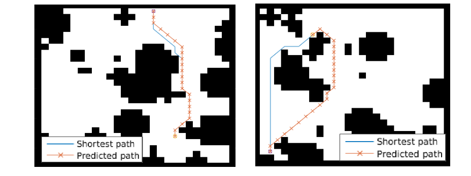
The agent gets a reward +1 in the goal state, -1 in obstacles (black), and -0.01 for each step (so that the shortest path to the goal is an optimal solution).
## VIN model
The agent is implemented in a very straight-forward manner as a single neural network trained with TRPO (Policy Gradients with a KL constraint on predictive action distributions over a batch of trajectories). So the only loss function used is to maximize expected reward, as is standard in model-free RL. However, the policy network of the agent has a very specific structure since it (internally) runs value iteration.
First, there's the core Value Iteration **(VI) Module** which runs the recurrence formula (reproducing again):

The input to this recurrence are the two arrays R (the reward array, reward for each state) and P (the dynamics array, the probabilities of transitioning to nearby states with each action), which are of course unknown to the agent, but can be predicted with neural networks as a function of the current state. This is a little funny because the networks take a _particular_ state **s** and are internally (during the forward pass) predicting the rewards and dynamics for all states and actions in the entire environment. Notice, extremely importantly and once again, that at no point are the reward and dynamics functions explicitly regressed to the observed transitions in the environment. They are just arrays of numbers that plug into value iteration recurrence module.
But anyway, once we have **R,P** arrays, in the Grid-world above due to the local connectivity, value iteration can be implemented with a repeated application of convolving **P** over **R**, as these filters effectively *diffuse* the estimated reward function (**R**) through the dynamics model (**P**), followed by max pooling across the actions. If **P** is a not a function of the state, it would simply be the filters in the Conv layer. Notice that posing this as convolution also assumes that the env dynamics are position-invariant. See the diagram below on the right: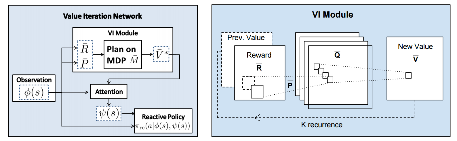
Once the array of numbers that we interpret as holding the estimated $V^*$ is computed after running **K** steps of the recurrence (K is fixed beforehand. For example for a 16x16 map it is 20, since that's a bit more than the amount of steps needed to diffuse rewards across the entire map), we "pluck out" the state-action values $Q(s,.)$ at the state the agent happens to currently be in (by an "attention" operator $\psi$), and (optionally) append these Q values to the feedforward representation of the current state $\phi(s)$, and finally predicting the action distribution.
## Experiments
**Baseline 1**: A vanilla ConvNet policy trained with TRPO. [(50 3x3 filters)\*2, 2x2 max pool, (100 3x3 filters)\*3, 2x2 max pool, FC(100), FC(4), Softmax].
**Baseline 2**: A fully convolutional network (FCN), 3 layers (with a filter that spans the whole image), of 150, 100, 10 filters. i.e. slightly different and perhaps a bit more domain-appropriate ConvNet architecture.
**Curriculum** is used during training where easier environments are trained on first. This is claimed to work better but not quantified in tables. Models are trained with TRPO, RMSProp, implemented in Theano.
Results when training on **5000** random grid-world instances (hey isn't that quite a bit low?):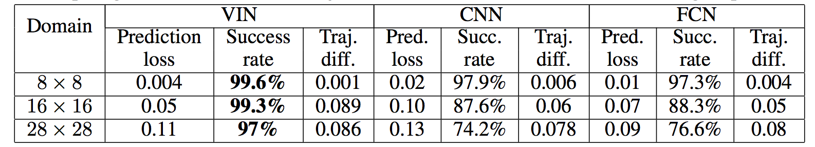
TLDR VIN generalizes better.
The authors also run the model on the **Mars Rover Navigation** dataset (wait what?), a **Continuous Control** 2D path planning dataset, and the **WebNav Challenge**, a language-based search task on a graph (of a subset of Wikipedia). Skipping these because they don't add _too_ much to the core cool idea of the paper.
## Misc
**The good**: I really like this paper because the core idea is cute (the planner is *embedded* in the policy and trained end-to-end), novel (I don't think I saw this idea executed on so far elsewhere), the paper is well-written and clear, and the supplementary materials are thorough.
**On the approach**: Significant challenges remain to make this approach more practicaly viable, but it also seems that much more exciting followup work can be done in this framework. I wish the authors discussed this more in the conclusion. In particular, it seems that one has to explicitly encode the environment connectivity structure in the internal model $\bar{M}$. How much of a problem is this and what could be done about it? Or how could we do the planning in more higher-level abstract spaces instead of the actual low-level state space of the problem? Also, it seems that a potentially nice feature of this approach is that the agent could dynamically "decide" on a reward function at runtime, and the VI module can diffuse it through the dynamics and hence do the planning. A potentially interesting outcome is that the agent could utilize this kind of computation so that an LSTM controller could learn to "emit" reward function subgoals and the VI planner computes how to meet them. A nice/clean division of labor one could hope for in principle.
**The experiments**. Unfortunately, I'm not sure why the authors preferred breadth of experiments and sacrificed depth of experiments. I would have much preferred a more in-depth analysis of the gridworld environment. For instance:
- Only 5,000 training examples are used for training, which seems very little. Presumable, the baselines get stronger as you increase the number of training examples?
- Lack of visualizations: Does the model actually learn the "correct" rewards **R** and dynamics **P**? The authors could inspect these manually and correlate them to the actual model. This would have been reaaaallllyy cool. I also wouldn't expect the model to exactly learn these, but who knows.
- How does the model compare to the baselines in the number of parameters? or FLOPS? It seems that doing VI for 30 steps at each single iteration of the algorithm should be quite expensive.
- The authors should study the performance as a function of the number of recurrences **K**. A particularly funny experiment would be K = 1, where the model would be effectively predicting **V*** directly, without planning. What happens?
- If the output of VI $\psi(s)$ is concatenated to the state parameters, are these Q values actually used? What if all the weights to these numbers are zero in the trained models?
- Why do the authors only evaluate success rate when the training criterion is expected reward?
Overall a very cute idea, well executed as a first step and well explained, with a bit of unsatisfying lack of depth in the experiments in favor of breadth that doesn't add all that much.
2 Comments
 |

Cooperative Inverse Reinforcement Learning
Hadfield-Menell, Dylan and Dragan, Anca and Abbeel, Pieter and Russell, Stuart J.
arXiv e-Print archive - 2016 via Local Bibsonomy
Keywords: dblp
Hadfield-Menell, Dylan and Dragan, Anca and Abbeel, Pieter and Russell, Stuart J.
arXiv e-Print archive - 2016 via Local Bibsonomy
Keywords: dblp
|
[link]
In the future, AI and people will work together; hence, we must concern ourselves with ensuring that AI will have interests aligned with our own. The authors suggest that it is in our best interests to find a solution to the "value-alignment problem". As recently pointed out by Ian Goodfellow, however, [this may not always be a good idea](https://www.quora.com/When-do-you-expect-AI-safety-to-become-a-serious-issue). Cooperative Inverse Reinforcement Learning (CIRL) is a formulation of a cooperative, partial information game between a human and a robot. Both share a reward function, but the robot does not initially know what it is. One of the key departures from classical Inverse Reinforcement Learning is that the teacher, which in this case is the human, is not assumed to act optimally. Rather, it is shown that sub-optimal actions on the part of the human can result in the robot learning a better reward function. The structure of the CIRL formulation is such that it should encourage the human to not attempt to teach by demonstration in a way that greedily maximizes immediate reward. Rather, the human learns how to "best respond" to the robot. CIRL can be formulated as a dec-POMDP, and reduced to a single-agent POMDP. The authors solved a 2D navigation task with CIRL to demonstrate the inferiority of having the human follow a "demonstration-by-expert" policy as opposed to a "best-response" policy. |

Matching Networks for One Shot Learning
Vinyals, Oriol and Blundell, Charles and Lillicrap, Timothy P. and Kavukcuoglu, Koray and Wierstra, Daan
arXiv e-Print archive - 2016 via Local Bibsonomy
Keywords: dblp
Vinyals, Oriol and Blundell, Charles and Lillicrap, Timothy P. and Kavukcuoglu, Koray and Wierstra, Daan
arXiv e-Print archive - 2016 via Local Bibsonomy
Keywords: dblp
|
[link]
Originally posted on my Github [paper-notes](https://github.com/karpathy/paper-notes/blob/master/matching_networks.md) repo.
# Matching Networks for One Shot Learning
By DeepMind crew: **Oriol Vinyals, Charles Blundell, Timothy Lillicrap, Koray Kavukcuoglu, Daan Wierstra**
This is a paper on **one-shot** learning, where we'd like to learn a class based on very few (or indeed, 1) training examples. E.g. it suffices to show a child a single giraffe, not a few hundred thousands before it can recognize more giraffes.
This paper falls into a category of *"duh of course"* kind of paper, something very interesting, powerful, but somehow obvious only in retrospect. I like it.
Suppose you're given a single example of some class and would like to label it in test images.
- **Observation 1**: a standard approach might be to train an Exemplar SVM for this one (or few) examples vs. all the other training examples - i.e. a linear classifier. But this requires optimization.
- **Observation 2:** known non-parameteric alternatives (e.g. k-Nearest Neighbor) don't suffer from this problem. E.g. I could immediately use a Nearest Neighbor to classify the new class without having to do any optimization whatsoever. However, NN is gross because it depends on an (arbitrarily-chosen) metric, e.g. L2 distance. Ew.
- **Core idea**: lets train a fully end-to-end nearest neighbor classifer!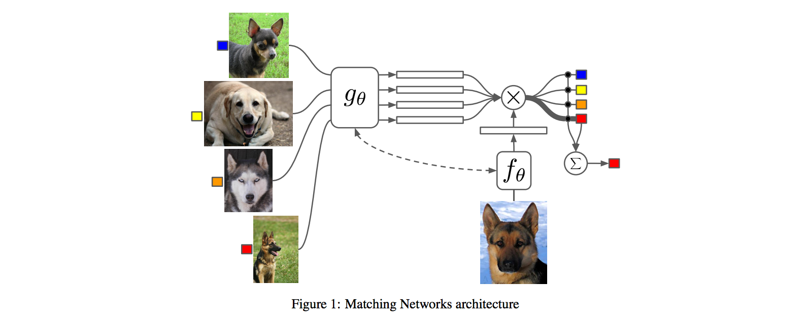
## The training protocol
As the authors amusingly point out in the conclusion (and this is the *duh of course* part), *"one-shot learning is much easier if you train the network to do one-shot learning"*. Therefore, we want the test-time protocol (given N novel classes with only k examples each (e.g. k = 1 or 5), predict new instances to one of N classes) to exactly match the training time protocol.
To create each "episode" of training from a dataset of examples then:
1. Sample a task T from the training data, e.g. select 5 labels, and up to 5 examples per label (i.e. 5-25 examples).
2. To form one episode sample a label set L (e.g. {cats, dogs}) and then use L to sample the support set S and a batch B of examples to evaluate loss on.
The idea on high level is clear but the writing here is a bit unclear on details, of exactly how the sampling is done.
## The model
I find the paper's model description slightly wordy and unclear, but basically we're building a **differentiable nearest neighbor++**. The output \hat{y} for a test example \hat{x} is computed very similar to what you might see in Nearest Neighbors:
where **a** acts as a kernel, computing the extent to which \hat{x} is similar to a training example x_i, and then the labels from the training examples (y_i) are weight-blended together accordingly. The paper doesn't mention this but I assume for classification y_i would presumbly be one-hot vectors.
Now, we're going to embed both the training examples x_i and the test example \hat{x}, and we'll interpret their inner products (or here a cosine similarity) as the "match", and pass that through a softmax to get normalized mixing weights so they add up to 1. No surprises here, this is quite natural:

Here **c()** is cosine distance, which I presume is implemented by normalizing the two input vectors to have unit L2 norm and taking a dot product. I assume the authors tried skipping the normalization too and it did worse? Anyway, now all that's left to define is the function **f** (i.e. how do we embed the test example into a vector) and the function **g** (i.e. how do we embed each training example into a vector?).
**Embedding the training examples.** This (the function **g**) is a bidirectional LSTM over the examples:
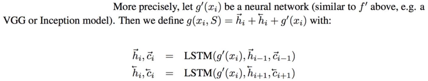
i.e. encoding of i'th example x_i is a function of its "raw" embedding g'(x_i) and the embedding of its friends, communicated through the bidirectional network's hidden states. i.e. each training example is a function of not just itself but all of its friends in the set. This is part of the ++ above, because in a normal nearest neighbor you wouldn't change the representation of an example as a function of the other data points in the training set.
It's odd that the **order** is not mentioned, I assume it's random? This is a bit gross because order matters to a bidirectional LSTM; you'd get different embeddings if you permute the examples.
**Embedding the test example.** This (the function **f**) is a an LSTM that processes for a fixed amount (K time steps) and at each point also *attends* over the examples in the training set. The encoding is the last hidden state of the LSTM. Again, this way we're allowing the network to change its encoding of the test example as a function of the training examples. Nifty: 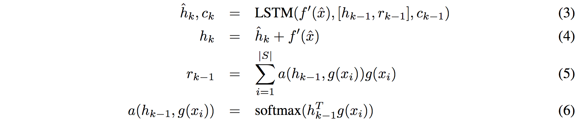
That looks scary at first but it's really just a vanilla LSTM with attention where the input at each time step is constant (f'(\hat{x}), an encoding of the test example all by itself) and the hidden state is a function of previous hidden state but also a concatenated readout vector **r**, which we obtain by attending over the encoded training examples (encoded with **g** from above).
Oh and I assume there is a typo in equation (5), it should say r_k = … without the -1 on LHS.
## Experiments
**Task**: N-way k-shot learning task. i.e. we're given k (e.g. 1 or 5) labelled examples for N classes that we have not previously trained on and asked to classify new instances into he N classes.
**Baselines:** an "obvious" strategy of using a pretrained ConvNet and doing nearest neighbor based on the codes. An option of finetuning the network on the new examples as well (requires training and careful and strong regularization!).
**MANN** of Santoro et al. [21]: Also a DeepMind paper, a fun NTM-like Meta-Learning approach that is fed a sequence of examples and asked to predict their labels.
**Siamese network** of Koch et al. [11]: A siamese network that takes two examples and predicts whether they are from the same class or not with logistic regression. A test example is labeled with a nearest neighbor: with the class it matches best according to the siamese net (requires iteration over all training examples one by one). Also, this approach is less end-to-end than the one here because it requires the ad-hoc nearest neighbor matching, while here the *exact* end task is optimized for. It's beautiful.
### Omniglot experiments
### 
Omniglot of [Lake et al. [14]](http://www.cs.toronto.edu/~rsalakhu/papers/LakeEtAl2015Science.pdf) is a MNIST-like scribbles dataset with 1623 characters with 20 examples each.
Image encoder is a CNN with 4 modules of [3x3 CONV 64 filters, batchnorm, ReLU, 2x2 max pool]. The original image is claimed to be so resized from original 28x28 to 1x1x64, which doesn't make sense because factor of 2 downsampling 4 times is reduction of 16, and 28/16 is a non-integer >1. I'm assuming they use VALID convs?
Results: 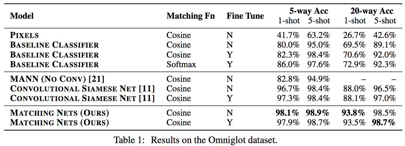
Matching nets do best. Fully Conditional Embeddings (FCE) by which I mean they the "Full Context Embeddings" of Section 2.1.2 instead are not used here, mentioned to not work much better. Finetuning helps a bit on baselines but not with Matching nets (weird).
The comparisons in this table are somewhat confusing:
- I can't find the MANN numbers of 82.8% and 94.9% in their paper [21]; not clear where they come from. E.g. for 5 classes and 5-shot they seem to report 88.4% not 94.9% as seen here. I must be missing something.
- I also can't find the numbers reported here in the Siamese Net [11] paper. As far as I can tell in their Table 2 they report one-shot accuracy, 20-way classification to be 92.0, while here it is listed as 88.1%?
- The results of Lake et al. [14] who proposed Omniglot are also missing from the table. If I'm understanding this correctly they report 95.2% on 1-shot 20-way, while matching nets here show 93.8%, and humans are estimated at 95.5%. That is, the results here appear weaker than those of Lake et al., but one should keep in mind that the method here is significantly more generic and does not make any assumptions about the existence of strokes, etc., and it's a simple, single fully-differentiable blob of neural stuff.
(skipping ImageNet/LM experiments as there are few surprises)
## Conclusions
Good paper, effectively develops a differentiable nearest neighbor trained end-to-end. It's something new, I like it!
A few concerns:
- A bidirectional LSTMs (not order-invariant compute) is applied over sets of training examples to encode them. The authors don't talk about the order actually used, which presumably is random, or mention this potentially unsatisfying feature. This can be solved by using a recurrent attentional mechanism instead, as the authors are certainly aware of and as has been discussed at length in [ORDER MATTERS: SEQUENCE TO SEQUENCE FOR SETS](https://arxiv.org/abs/1511.06391), where Oriol is also the first author. I wish there was a comment on this point in the paper somewhere.
- The approach also gets quite a bit slower as the number of training examples grow, but once this number is large one would presumable switch over to a parameteric approach.
- It's also potentially concerning that during training the method uses a specific number of examples, e.g. 5-25, so this is the number of that must also be used at test time. What happens if we want the size of our training set to grow online? It appears that we need to retrain the network because the encoder LSTM for the training data is not "used to" seeing inputs of more examples? That is unless you fall back to iteratively subsampling the training data, doing multiple inference passes and averaging, or something like that. If we don't use FCE it can still be that the attention mechanism LSTM can still not be "used to" attending over many more examples, but it's not clear how much this matters. An interesting experiment would be to not use FCE and try to use 100 or 1000 training examples, while only training on up to 25 (with and fithout FCE). Discussion surrounding this point would be interesting.
- Not clear what happened with the Omniglot experiments, with incorrect numbers for [11], [21], and the exclusion of Lake et al. [14] comparison.
- A baseline that is missing would in my opinion also include training of an [Exemplar SVM](https://www.cs.cmu.edu/~tmalisie/projects/iccv11/), which is a much more powerful approach than encode-with-a-cnn-and-nearest-neighbor.
4 Comments
 |
Deep Image Retrieval: Learning global representations for image search
Gordo, Albert and Almazán, Jon and Revaud, Jérome and Larlus, Diane
arXiv e-Print archive - 2016 via Local Bibsonomy
Keywords: dblp
Gordo, Albert and Almazán, Jon and Revaud, Jérome and Larlus, Diane
arXiv e-Print archive - 2016 via Local Bibsonomy
Keywords: dblp
|
[link]
**Contributions:** - Triplet ranking loss, implemented in three-stream Siamese network - Integrate region proposal network in system. All operations are derivative, making the system end-to-end trainable. - Proposed dataset cleaning method, which is critical for performance boost. - Performance surpasses previous global descriptors and most of local based descriptors in Landmarks dataset. **Training:** - Sample triplets, triplet hinge loss: $L(I_q, I^+, I^-)=max(0, m+q^Td^- - q^Td^+)$ - Since only convolutional layers are used in CNN, and aggregation does not require a fixed input size, full image resolution could be used. **Network data flow:** - Use convolutional layers of pre-trained network to extract activation features. - Max-pooling in different regions, using multi-scale rigid grid with overlapping cells. Note that ROI pooling is differentiable. - L2 normalize region features, whiten with PCA and l2-normalize again. PCA projection can be implemented with a shifting and a FC layer. - Aggregate: sum and l2 normalize. - Dot product similarity of image vector is approximately many-to-many region matching. **Region Proposal Network** - Objective function is multi-task loss, which combines classification loss and regression loss. - When applied, need to perform non-maximum suppression, keep top K proposals for each image. **Landmark Dataset Cleaning** - Construct image graph, with edges as similarity score. The score is computed offline, using invariant keypoint matching and spatial verification. - Extract connected components in graph. They correspond to differnt profiles of a landmark. |

Density estimation using Real NVP
Laurent Dinh and Jascha Sohl-Dickstein and Samy Bengio
arXiv e-Print archive - 2016 via Local arXiv
Keywords: cs.LG
First published: 2016/05/27 (8 years ago)
Abstract: Unsupervised learning of probabilistic models is a central yet challenging problem in machine learning. Specifically, designing models with tractable learning, sampling, inference and evaluation is crucial in solving this task. We extend the space of such models using real-valued non-volume preserving (real NVP) transformations, a set of powerful invertible and learnable transformations, resulting in an unsupervised learning algorithm with exact log-likelihood computation, exact sampling, exact inference of latent variables, and an interpretable latent space. We demonstrate its ability to model natural images on four datasets through sampling, log-likelihood evaluation and latent variable manipulations.
more
less
Laurent Dinh and Jascha Sohl-Dickstein and Samy Bengio
arXiv e-Print archive - 2016 via Local arXiv
Keywords: cs.LG
First published: 2016/05/27 (8 years ago)
Abstract: Unsupervised learning of probabilistic models is a central yet challenging problem in machine learning. Specifically, designing models with tractable learning, sampling, inference and evaluation is crucial in solving this task. We extend the space of such models using real-valued non-volume preserving (real NVP) transformations, a set of powerful invertible and learnable transformations, resulting in an unsupervised learning algorithm with exact log-likelihood computation, exact sampling, exact inference of latent variables, and an interpretable latent space. We demonstrate its ability to model natural images on four datasets through sampling, log-likelihood evaluation and latent variable manipulations.
|
[link]
This paper presents a novel neural network approach (though see [here](https://www.facebook.com/hugo.larochelle.35/posts/172841743130126?pnref=story) for a discussion on prior work) to density estimation, with a focus on image modeling. At its core, it exploits the following property on the densities of random variables. Let $x$ and $z$ be two random variables of equal dimensionality such that $x = g(z)$, where $g$ is some bijective and deterministic function (we'll note its inverse as $f = g^{-1}$). Then the change of variable formula gives us this relationship between the densities of $x$ and $z$:

$p_X(x) = p_Z(z) \left|{\rm det}\left(\frac{\partial g(z)}{\partial z}\right)\right|^{-1}$

Moreover, since the determinant of the Jacobian matrix of the inverse $f$ of a function $g$ is simply the inverse of the Jacobian of the function $g$, we can also write:

$p_X(x) = p_Z(f(x)) \left|{\rm det}\left(\frac{\partial f(x)}{\partial x}\right)\right|$

where we've replaced $z$ by its deterministically inferred value $f(x)$ from $x$.

So, the core of the proposed model is in proposing a design for bijective functions $g$ (actually, they design its inverse $f$, from which $g$ can be derived by inversion), that have the properties of being easily invertible and having an easy-to-compute determinant of Jacobian. Specifically, the authors propose to construct $f$ from various modules that all preserve these properties and allows to construct highly non-linear $f$ functions. Then, assuming a simple choice for the density $p_Z$ (they use a multidimensional Gaussian), it becomes possible to both compute $p_X(x)$ tractably and to sample from that density, by first samples $z\sim p_Z$ and then computing $x=g(z)$.

The building blocks for constructing $f$ are the following:

**Coupling layers**: This is perhaps the most important piece. It simply computes as its output $b\odot x + (1-b) \odot (x \odot \exp(l(b\odot x)) + m(b\odot x))$, where $b$ is a binary mask (with half of its values set to 0 and the others to 1) over the input of the layer $x$, while $l$ and $m$ are arbitrarily complex neural networks with input and output layers of equal dimensionality.

In brief, for dimensions for which $b_i = 1$ it simply copies the input value into the output. As for the other dimensions (for which $b_i = 0$) it linearly transforms them as $x_i * \exp(l(b\odot x)_i) + m(b\odot x)_i$. Crucially, the bias ($m(b\odot x)_i$) and coefficient ($\exp(l(b\odot x)_i)$) of the linear transformation are non-linear transformations (i.e. the output of neural networks) that only have access to the masked input (i.e. the non-transformed dimensions). While this layer might seem odd, it has the important property that it is invertible and the determinant of its Jacobian is simply $\exp(\sum_i (1-b_i) l(b\odot x)_i)$. See Section 3.3 for more details on that.

**Alternating masks**: One important property of coupling layers is that they can be stacked (i.e. composed), and the resulting composition is still a bijection and is invertible (since each layer is individually a bijection) and has a tractable determinant for its Jacobian (since the Jacobian of the composition of functions is simply the multiplication of each function's Jacobian matrix, and the determinant of the product of square matrices is the product of the determinant of each matrix). This is also true, even if the mask $b$ of each layer is different. Thus, the authors propose using masks that alternate across layer, by masking a different subset of (half of) the dimensions. For images, they propose using masks with a checkerboard pattern (see Figure 3). Intuitively, alternating masks are better because then after at least 2 layers, all dimensions have been transformed at least once.

**Squeezing operations**: Squeezing operations corresponds to a reorganization of a 2D spatial layout of dimensions into 4 sets of features maps with spatial resolutions reduced by half (see Figure 3). This allows to expose multiple scales of resolutions to the model. Moreover, after a squeezing operation, instead of using a checkerboard pattern for masking, the authors propose to use a per channel masking pattern, so that "the resulting partitioning is not redundant with the previous checkerboard masking". See Figure 3 for an illustration.

Overall, the models used in the experiments usually stack a few of the following "chunks" of layers: 1) a few coupling layers with alternating checkboard masks, 2) followed by squeezing, 3) followed by a few coupling layers with alternating channel-wise masks. Since the output of each layers-chunk must technically be of the same size as the input image, this could become expensive in terms of computations and space when using a lot of layers. Thus, the authors propose to explicitly pass on (copy) to the very last layer ($z$) half of the dimensions after each layers-chunk, adding another chunk of layers only on the other half. This is illustrated in Figure 4b.

Experiments on CIFAR-10, and 32x32 and 64x64 versions of ImageNet show that the proposed model (coined the real-valued non-volume preserving or Real NVP) has competitive performance (in bits per dimension), though slightly worse than the Pixel RNN.

**My Two Cents**

The proposed approach is quite unique and thought provoking. Most interestingly, it is the only powerful generative model I know that combines A) a tractable likelihood, B) an efficient / one-pass sampling procedure and C) the explicit learning of a latent representation. While achieving this required a model definition that is somewhat unintuitive, it is nonetheless mathematically really beautiful!

I wonder to what extent Real NVP is penalized in its results by the fact that it models pixels as real-valued observations. First, it implies that its estimate of bits/dimensions is an upper bound on what it could be if the uniform sub-pixel noise was integrated out (see Equations 3-4-5 of [this paper](http://arxiv.org/pdf/1511.01844v3.pdf)). Moreover, the authors had to apply a non-linear transformation (${\rm logit}(\alpha + (1-\alpha)\odot x)$) to the pixels, to spread the $[0,255]$ interval further over the reals. Since the Pixel RNN models pixels as discrete observations directly, the Real NVP might be at a disadvantage.

I'm also curious to know how easy it would be to do conditional inference with the Real NVP. One could imagine doing approximate MAP conditional inference, by clamping the observed dimensions and doing gradient descent on the log-likelihood with respect to the value of remaining dimensions. This could be interesting for image completion, or for structured output prediction with real-valued outputs in general. I also wonder how expensive that would be.

In all cases, I'm looking forward to saying interesting applications and variations of this model in the future!
|
A Model Explanation System: Latest Updates and Extensions
Turner, Ryan
arXiv e-Print archive - 2016 via Local Bibsonomy
Keywords: dblp
Turner, Ryan
arXiv e-Print archive - 2016 via Local Bibsonomy
Keywords: dblp
|
[link]
#### Explainability-Accuracy trade-off Many practical applications of machine learning systems call for the ability to explain why certain predictions are made. Consider a fraud detection system: it is not very useful for a user to see a list of possible fraud attempts without any explanation why the system thought the attempt was fraud. You want to say something like 'the system thinks it's fraud because the credit card was used to make several transactions that are smaller than usual'. But such explanations are not always compatible with our machine learning model. Or are they? When choosing a machine learning model we usually think in terms of two choices: - accurate but black-box: The best classification accuracy is typically achieved by black-box models such as Gaussian processes, neural networks or random forests, or complicated ensembles of all of these. Just look at the kaggle leaderboards. These are called black-box and are often criticised because their inner workings are really hard to understand. They don't, in general, provide a clear explanation of the reasons they made a certain prediction, they just spit out a probability. - white-box but weak: On the other end of the spectrum, models whose predictions are easy to understand and communicate are usually very impoverished in their predictive capacity (linear regression, a single decision tree) or are inflexible and computationally cumbersome (explicit graphical models). So which ones should we use: accurate black-box models, or less accurate but easy-to-explain white-box models? The paper basically tells us that this is a false tradeoff. To summarise my take-home from this poster in one sentence: `Explainability is not a property of the model` Ryan presents a nice way to separate concerns of predictive power and explanation generation. He does this by introducing a formal framework in which simple, human-readable explanations can be generated for any black-box classifier, without assuming anything about the internal workings of the classifier. If you think about it, it makes sense. If you watch someone playing chess, you can probably post-rationalise and give a reason why the person might think it's a good move. But you probably don't have an idea about the algorithm the person was executing in his brain. Now we have a way to explain why decisions were made by complex systems, even if that explanation is not an exact explanation of what the classifier algorithm actually did. This is super-important in applications such as face recognitions where the only models that seem to work today are large black-box models. As (buzzword alert) AI-assisted decision making is becoming commonplace, the ability to generate simple explanations for black-box systems is going to be super important, and I think Ryan has made some very good observations in this paper. I recommend everyone to take a look, I'm definitely going to see the world a bit differently after reading this. |

Unsupervised Learning of Visual Representations by Solving Jigsaw Puzzles
Noroozi, Mehdi and Favaro, Paolo
arXiv e-Print archive - 2016 via Local Bibsonomy
Keywords: dblp
Noroozi, Mehdi and Favaro, Paolo
arXiv e-Print archive - 2016 via Local Bibsonomy
Keywords: dblp
|
[link]
The core idea behind this paper is powerfully simple. The goal is to learn useful representations from unlabelled data, useful in the sense of helping supervised object classification. This paper does this by chopping up images into a set of little jigsaw puzzle, scrambling the pieces, and asking a deep neural network to learn to reassemble them in the correct constellation. A picture is worth a thousand words, so here is Figure 1 taken from the paper explaining this visually:
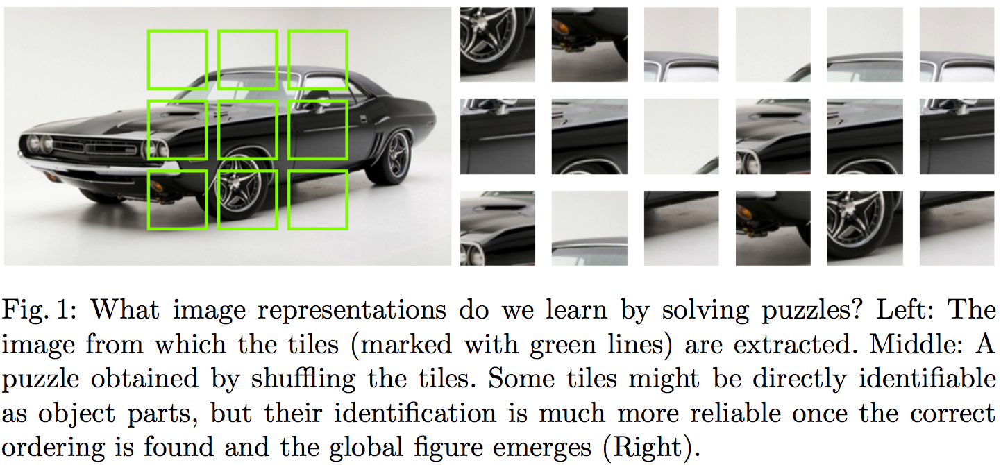
#### Summary of this note:
- I note the similarities to denoising autoencoders, which motivate my question: "Can this method equivalently represent the data generating distribution?"
- I consider a toy example with just two jigsaw pieces, and consider using an objective like this to fit a generative model $Q$ to data
- I show how the jigsaw puzzle training procedure corresponds to minimising a difference of KL divergences
- Conclude that the algorithm ignores some aspects of the data generating distribution, and argue that in this case it can be a good thing
#### What does this learn do?
This idea seems to make a lot of sense. But to me, one interesting question is the following:
`What does a network trained to solve jigsaw puzzle learn about the data generating distribution?`
#### Motivating example: denoising autoencoders
At one level, this jigsaw puzzle approach bears similarities to denoising autoencoders (DAEs): both methods are self-supervised: they take an unlabelled data and generate a synthetic supervised learning task. You can also interpret solving jigsaw puzzles as a special case 'undoing corruption' thus fitting a more general definition of autoencoders (Bengio et al, 2014).
DAEs have been shown to be related to score matching (Vincent, 2000), and that they learn to represent gradients of the log-probability-density-function of the data generating distribution (Alain et al, 2012). In this sense, autoencoders equivalently represent a complete probability distribution up to normalisation. This concept is also exploited in Harri Valpola's work on ladder networks (Rasmus et al, 2015)
So I was curious if I can find a similar neat interpretation of what really is going on in this jigsaw puzzle thing. If you equivalently represent all aspects of a probability distribution this way? Are there aspects that this representation ignores? Would it correspond to a consistent denisty estimation/generative modelling method in any sense? Below is my attempt to figure this out.
#### A toy case with just two jigsaw pieces
To simplify things, let's just consider a simpler jigsaw puzzle problem with just two jigsaw positions instead of 9, and in such a way that there are no gaps between puzzle pieces, so image patches (now on referred to as data $x$) can be partitioned exactly into pieces.
Let's assume our datapoints $x^{(n)}$ are drawn i.i.d. from an unknown distribution $P$, and that $x$ can be partitioned into two chunks $x_1$ and $x_2$ of equivalent dimensionality, such that $x=(x_1,x_2)$ by definition. Let's also define the permuted/scrambled version of a datapoint $x$ as $\hat{x}:=(x_2,x_1)$.
The jigsaw puzzle problem can be formulated in the following way: we draw a datapoint $x$ from $P$. We also independently draw a binary 'label' $y$ from a Bernoulli($\frac{1}{2}$) distribution, i.e. toss a coin. If $y=1$ we set $z=x$ otherwise $z=\hat{x}$.
Our task is to build a predictior, $f$, which receives as input $z$ and infers the value of $y$ (outputs the probability that its value is $1$). In other words, $f$ tries to guess the correct ordering of the chunks that make up the randomly scrambled datapoint $z$, thereby solving the jigsaw puzzle. The accuracy of the predictor is evaluated using the log-loss, a.k.a. binary cross-entropy, as it is common in binary classification problems:
$$ \mathcal{L}(f) = - \frac{1}{2} \mathbb{E}_{x\sim P} \left[\log f(x) + \log (1 - f(\hat{x}))\right] $$
Let's consider the case when we express the predictor $f$ in terms of a generative model $Q$ of $x$. $Q$ is an approximation to $P$, and has some parameters $\theta$ which we can tweak. For a given $\theta$, the posterior predictive distribution of $y$ takes the following form:
$$ f(z,\theta) := Q(y=1\vert z;\theta) = \frac{Q(z;\theta)}{Q(z;\theta) + Q(\hat{z};\theta)},
$$
where $\hat{z}$ denotes the scrambled/permuted version of $z$. Notice that when $f$ is defined this way the following property holds:
$$ 1 - f(\hat{x};\theta) = f(x;\theta),
$$
so we can simplify the expression for the log-loss to finally obtain:
\begin{align} \mathcal{L}(\theta) &= - \mathbb{E}_{x \sim P} \log Q(x;\theta) + \mathbb{E}_{x \sim P} \log [Q(x;\theta) + Q(\hat{x};\theta)]\\ &= \operatorname{KL}[P\|Q_{\theta}] - \operatorname{KL}\left[P\middle\|\frac{Q_{\theta}(x)+Q_{\theta}(\hat{x})}{2}\right] + \log(2) \end{align}
So we already see that using the jigsaw objective to train a generative model reduces to minimising the difference between two KL divergences. It's also possible to reformulate the loss as:
$$ \mathcal{L}(\theta) = \operatorname{KL}[P\|Q_{\theta}] - \operatorname{KL}\left[\frac{P(x) + P(\hat{x})}{2}\middle\|\frac{Q_{\theta}(x)+Q_{\theta}(\hat{x})}{2}\right] - \operatorname{KL}\left[P\middle\|\frac{P(x) + P(\hat{x})}{2}\right] + \log(2) $$
Let's look at what the different terms do:
- The first term is the usual KL divergence that would correspond to maximum likelihood. So it just tries to make $Q$ as close to $P$ as possible.
- The second term is a bit weird, particularly as comes into the formula with a negative sign. The KL divergence is $0$ if $Q$ and $P$ define the distribution over the set of jigsaw pieces ${x_1,x_2}$. Notice, I used set notation here, so the ordering does not matter. In a way this term tells the loss function: don't bother modelling what the jigsaw pieces are, only model how they fit together.
- The last terms are constant wrt. $\theta$ so we don't need to worry about them.
#### Not a proper scoring rule (and it's okay)
From the formula above it is clear that the jigsaw training objective wouldn't be a proper scoring rule, as it is not uniquely minimised by $Q=P$ in all cases. Here are two counterexamples where the objective fails to capture all aspects of $P$:
Consider the case when $P=\frac{P(x) + P(\hat{x})}{2}$, that is, when $P$ is completely insensitive to the ordering of jigsaw pieces. As long as $Q$ also has this property $Q = \frac{Q(x) + Q(\hat{x})}{2}$, all KL divergences are $0$ and the jigsaw objective is constant with respect $\theta$. Indeed, it is impossible in this case for any classifier to surpass chance level in the jigsaw problem.
Another simple example to consider is a two-dimensional binary $P$. Here, the jigsaw objective only cares about the value of $Q(0,1)$ relative to $Q(1,0)$, but completely insensitive to $Q(1,1)$ and $Q(0,0)$. In other words, we don't really care how often $0$s and $1$s appear, we just want to know which one is likelier to be on the left or the right side.
This is all fine because we don't use this technique for generative modelling. We want to use it for representation learning, so it's okay to ignore some aspects of $P$.
#### Representation learning
I think this method seems like a really promising direction for unsupervised representation learning. In my mind representation learning needs either:
- strong prior assumptions about what variables/aspects of data are behaviourally relevant, or relevant to the tasks we want to solve with the representations.
- at least a little data in a semi-supervised setting to inform us about what is relevant and what is not.
Denoising autoencoders (with L2 reconstruction loss) and maximum likelihood training try to represent all aspects of the data generating distribution, down to pixel level. We can encode further priors in these models in various ways, either by constraining the network architecture or via probabilistic priors over latent variables.
The jigsaw method encodes prior assumptions into the training procedure: that the structure of the world (relative position of parts) is more important to get right than the low-level appearance of parts. This is probably a fair assumption.
|
Unsupervised Feature Extraction by Time-Contrastive Learning and Nonlinear ICA
Hyvärinen, Aapo and Morioka, Hiroshi
arXiv e-Print archive - 2016 via Local Bibsonomy
Keywords: dblp
Hyvärinen, Aapo and Morioka, Hiroshi
arXiv e-Print archive - 2016 via Local Bibsonomy
Keywords: dblp
|
[link]
"Aapo did it again!" - I exclaimed while reading this paper yesterday on the train back home (or at least I thought I was going home until I realised I was sitting on the wrong train the whole time. This gave me a couple more hours to think while traveling on a variety of long-distance buses...) Aapo Hyvärinen is one of my heroes - he did tons of cool work, probably most famous for pseudo-likelihood, score matching and ICA. His recent paper, brought to my attention by my brand new colleague Hugo Larochelle, is similarly excellent: ### Summary Time-contrastive learning (TCL) trains a classifier that looks at a datapoint and guesses what part of the time series it came from. it exploits nonstationarity of time series to help representation learning an elegant connection to generative models (nonlinear ICA) is shown, although the assumptions of the model are pretty limiting TCL is the temporal analogue of representation learning with jigsaw puzzles similarly to GANs, logistic regression is deployed as a proxy to learn log-likelihood ratios directly from data Time-contrastive learning Time-contrastive learning (TCL) is a technique for learning to extract nonlinear representations from time series data. First, the time series is sliced up into a number of non-overlapping chunks, indexed by ττ. Then, a multivariate logistic regression classifier is trained in a supervised manner to look at a sample taken from the series at an unknown time and predict ττ, the index of the chunk it came from. For this classifier, a neural network is used. The classifier itself is only a proxy to solving the representation learning problem. It turns out, if you chop off the final linear + softmax layer, the activations in the last hidden layer will learn to represent something fundamental, the log-odds-ratios in a probabilistic generative model (see paper for details). If one runs linear ICA over these hidden layer activations, the resulting network will learn to perform inference in a nonlinear ICA latent variable model. Moreover, if certain conditions about nonstationarity and the generative model are met, one can prove that the latent variable model is identifiable. This means that if the data was indeed drawn from the nonlinear ICA generative model, the resulting inference network - composed by the chopping off the top of the classifier and replacing it with a linear ICA layer - can infer the true hidden variables exactly. ### How practical are the assumptions? TCL relies on the nonstationarity of time series data: the statistics of data changes depending on which chunk or slice of the time series you are in, but it is also assumed that data are i.i.d. within each chunk. The proof also assumes that the chunk-conditional data distributions are slightly modulated versions of the same nonlinear ICA generative model, this is how the model ends up identifiable - because we can use the different temporal chunks as different perspectives on the latent variables. I would say that these assumptions are not very practical, or at least on data such as natural video. Something along the lines of slow-feature analysis, with latent variables that exhibit more interesting behaviour over time would be desirable. Nevertheless, the model is complex enough to make a point, and I beleive TCL itself can be deployed more generally for representation learning. ### Temporal jigsaw It's not hard to see that TCL is analogous to a temporal version of the jigsaw puzzle method I wrote about last month. In the jigsaw puzzle method, one breaks up a single image into non-overlapping chunks, shuffles them, and then trains a network to reassemble the pieces. Here, the chunking happens in the temporal domain instead. There are other papers that use the same general idea: training classifiers that guess the correct temporal ordering of frames or subsequences in videos. To do well at their job, these classifiers can end up learning about objects, motion, perhaps even a notion of inertia, gravity or causality. Ishan Misra et al. (2016) Unsupervised Learning using Sequential Verification for Action Recognition Basura Fernando et al. (2015) Modeling Video Evolution For Action Recognition In this context, the key contribution of Hyvarinen and Morioka's paper is to provide extra theoretical justification, and relating the idea to generative models. I'm sure one can use this framework to extend TCL to slightly more plausible generative models. ### Key takeaway `Logistic regression learns likelihood ratios` This is yet another example of using logistic regression as a proxy to estimating log-probability-ratios directly from data. The same thing happens in generative adversarial networks, where the discriminator learns to represent $\log P(x) - \log Q(x)$, where $P$ and $Q$ are the real and synthetic data distributions, respectively. This insight provides new ways in which unsupervised or semi-supervised tasks can be reduced to supervised learning problems. As classification is now considered significantly easier than density estimation, direct probability ratio estimation may provide the easiest path forward for representation learning. |
A Convolutional Attention Network for Extreme Summarization of Source Code
Allamanis, Miltiadis and Peng, Hao and Sutton, Charles A.
arXiv e-Print archive - 2016 via Local Bibsonomy
Keywords: dblp
Allamanis, Miltiadis and Peng, Hao and Sutton, Charles A.
arXiv e-Print archive - 2016 via Local Bibsonomy
Keywords: dblp
|
[link]
[web site](http://groups.inf.ed.ac.uk/cup/codeattention/), [code (Theano)](https://github.com/mast-group/convolutional-attention), [working version of code](https://github.com/udibr/convolutional-attention), [ICML](http://icml.cc/2016/?page_id=1839#971), [external notes](https://github.com/jxieeducation/DIY-Data-Science/blob/master/papernotes/2016/02/conv-attention-network-source-code-summarization.md)
Given an arbitrary snippet of Java code (~72 tokens) generate the methods name (~3 tokens):
generation starts with a $m_0 = \text{start-symbol}$ and state $h_0$, to generate next output token $m_t$ do:
* convert code tokens $c_i$ and embed to $E_{c_i}$
* convert all $E_{c_i}$ to $\alpha$ and $\kappa$ all same length as code using a network of `Conv1D` and padding (`Conv1D` because the code is highly structured, unambiguous.) The convertion is done using following network:

* $\alpha$ and $\kappa$ are probabilities over length of code (using softmax).
* In addition compute $\lambda$ by running another `Conv1D` over $L_\text{feat}$ with $\sigma$ activation and take the maximal value.
* use $\alpha$ to weight average $E_{c_i}$ and pass the average through FC layer to end with a softmax over output vocabulary $V$. Probability for output word $m_t$ is $n_{m_t}$.
* As an alternative use $\kappa$ to give probability to use as output each of the tokens $c_i$ which can be inside $V$ or outside it. This is also called "translation-invariant features" ([ref](https://papers.nips.cc/paper/5866-pointer-networks.pdf))
* $\lambda$ is used as a meta-attention deciding which to use:
$P(m_t \mid h_{t-1},c) = \lambda \sum_i \kappa_i I_{c_i = m_t} + (1-\lambda) \mu n_{m_t}$
where $\mu$ is $1$ unless you are in training and $m_t$ is UNK and the correct value for $m_t$ appears in $c$ in which case it is $e^{-10}$
* Advance $h_{t-1}$ to $h_t$ with GRU and using as input the embedding of output token $m_{t-1}$ (while training this is taken from the training labels or with small probability the argmax of the generated output.)
* Generating using hybrid breadth-first search and beam search: keep a heap of all suggestions and always try to extend the best suggestion so far. Remove suggestions that are worse than all the completed suggestions (dead) so far.
|
Recurrent Highway Networks
Julian Georg Zilly and Rupesh Kumar Srivastava and Jan Koutník and Jürgen Schmidhuber
arXiv e-Print archive - 2016 via Local arXiv
Keywords: cs.LG, cs.CL, cs.NE
First published: 2016/07/12 (8 years ago)
Abstract: Many sequential processing tasks require complex nonlinear transition functions from one step to the next. However, recurrent neural networks with such 'deep' transition functions remain difficult to train, even when using Long Short-Term Memory networks. We introduce a novel theoretical analysis of recurrent networks based on Ger\v{s}gorin's circle theorem that illuminates several modeling and optimization issues and improves our understanding of the LSTM cell. Based on this analysis we propose Recurrent Highway Networks (RHN), which are long not only in time but also in space, generalizing LSTMs to larger step-to-step depths. Experiments indicate that the proposed architecture results in complex but efficient models, beating previous models for character prediction on the Hutter Prize dataset with less than half of the parameters.
more
less
Julian Georg Zilly and Rupesh Kumar Srivastava and Jan Koutník and Jürgen Schmidhuber
arXiv e-Print archive - 2016 via Local arXiv
Keywords: cs.LG, cs.CL, cs.NE
First published: 2016/07/12 (8 years ago)
Abstract: Many sequential processing tasks require complex nonlinear transition functions from one step to the next. However, recurrent neural networks with such 'deep' transition functions remain difficult to train, even when using Long Short-Term Memory networks. We introduce a novel theoretical analysis of recurrent networks based on Ger\v{s}gorin's circle theorem that illuminates several modeling and optimization issues and improves our understanding of the LSTM cell. Based on this analysis we propose Recurrent Highway Networks (RHN), which are long not only in time but also in space, generalizing LSTMs to larger step-to-step depths. Experiments indicate that the proposed architecture results in complex but efficient models, beating previous models for character prediction on the Hutter Prize dataset with less than half of the parameters.
|
[link]
multi layer RNN in which first layer is LSTM, following layers $l$ have $t$,$c$ gates that control whether the state of the layer is carried from previous state or transferred previous layer:
$s_l^{[t]} = h_l^{[t]} \cdot t_l^{[t]} + s_{l-1}^{[t]} \cdot c
_l^{[t]}$
|
Learning Representations for Counterfactual Inference
Johansson, Fredrik D. and Shalit, Uri and Sontag, David
arXiv e-Print archive - 2016 via Local Bibsonomy
Keywords: dblp
Johansson, Fredrik D. and Shalit, Uri and Sontag, David
arXiv e-Print archive - 2016 via Local Bibsonomy
Keywords: dblp
|
[link]
This paper presents a method to train a neural network to make predictions for *counterfactual* questions. In short, such questions are questions about what the result of an intervention would have been, had a different choice for the intervention been made (e.g. *Would this patient have lower blood sugar had she received a different medication?*).

One approach to tackle this problem is to collect data of the form $(x_i, t_i, y_i^F)$ where $x_i$ describes a situation (e.g. a patient), $t_i$ describes the intervention made (in this paper $t_i$ is binary, e.g. $t_i = 1$ if a new treatment is used while $t_i = 0$ would correspond to using the current treatment) and $y_i^F$ is the factual outcome of the intervention $t_i$ for $x_i$. From this training data, a predictor $h(x,t)$ taking the pair $(x_i, t_i)$ as input and outputting a prediction for $y_i^F$ could be trained.

From this predictor, one could imagine answering counterfactual questions by feeding $(x_i, 1-t_i)$ (i.e. a description of the same situation $x_i$ but with the opposite intervention $1-t_i$) to our predictor and comparing the prediction $h(x_i, 1-t_i)$ with $y_i^F$. This would give us an estimate of the change in the outcome, had a different intervention been made, thus providing an answer to our counterfactual question.

The authors point out that this scenario is related to that of domain adaptation (more specifically to the special case of covariate shift) in which the input training distribution (here represented by inputs $(x_i,t_i)$) is different from the distribution of inputs that will be fed at test time to our predictor (corresponding to the inputs $(x_i, 1-t_i)$). If the choice of intervention $t_i$ is evenly spread and chosen independently from $x_i$, the distributions become the same. However, in observational studies, the choice of $t_i$ for some given $x_i$ is often not independent of $x_i$ and made according to some unknown policy. This is the situation of interest in this paper.

Thus, the authors propose an approach inspired by the domain adaptation literature. Specifically, they propose to have the predictor $h(x,t)$ learn a representation of $x$ that is indiscriminate of the intervention $t$ (see Figure 2 for the proposed neural network architecture). Indeed, this is a notion that is [well established][1] in the domain adaptation literature and has been exploited previously using regularization terms based on [adversarial learning][2] and [maximum mean discrepancy][3]. In this paper, the authors used instead a regularization (noted in the paper as $disc(\Phi_{t=0},\Phi_ {t=1})$) based on the so-called discrepancy distance of [Mansour et al.][4], adapting its use to the case of a neural network.

As an example, imagine that in our dataset, a new treatment ($t=1$) was much more frequently used than not ($t=0$) for men. Thus, for men, relatively insufficient evidence for counterfactual inference is expected to be found in our training dataset. Intuitively, we would thus want our predictor to not rely as much on that "feature" of patients when inferring the impact of the treatment.

In addition to this term, the authors also propose incorporating an additional regularizer where the prediction $h(x_i,1-t_i)$ on counterfactual inputs is pushed to be as close as possible to the target $y_{j}^F$ of the observation $x_j$ that is closest to $x_i$ **and** actually had the counterfactual intervention $t_j = 1-t_i$.

The paper first shows a bound relating the counterfactual generalization error to the discrepancy distance. Moreover, experiments simulating counterfactual inference tasks are presented, in which performance is measured by comparing the predicted treatment effects (as estimated by the difference between the observed effect $y_i^F$ for the observed treatment and the predicted effect $h(x_i, 1-t_i)$ for the opposite treatment) with the real effect (known here because the data is simulated). The paper shows that the proposed approach using neural networks outperforms several baselines on this task.

**My two cents**

The connection with domain adaptation presented here is really clever and enlightening. This sounds like a very compelling approach to counterfactual inference, which can exploit a lot of previous work on domain adaptation.

The paper mentions that selecting the hyper-parameters (such as the regularization terms weights) in this scenario is not a trivial task. Indeed, measuring performance here requires knowing the true difference in intervention outcomes, which in practice usually cannot be known (e.g. two treatments usually cannot be given to the same patient once). In the paper, they somewhat "cheat" by using the ground truth difference in outcomes to measure out-of-sample performance, which the authors admit is unrealistic. Thus, an interesting avenue for future work would be to design practical hyper-parameter selection procedures for this scenario. I wonder whether the *reverse cross-validation* approach we used in our work on our adversarial approach to domain adaptation (see [Section 5.1.2][5]) could successfully be used here.

Finally, I command the authors for presenting such a nicely written description of counterfactual inference problem setup in general, I really enjoyed it!

[1]: https://papers.nips.cc/paper/2983-analysis-of-representations-for-domain-adaptation.pdf
[2]: http://arxiv.org/abs/1505.07818
[3]: http://ijcai.org/Proceedings/09/Papers/200.pdf
[4]: http://www.cs.nyu.edu/~mohri/pub/nadap.pdf
[5]: http://arxiv.org/pdf/1505.07818v4.pdf#page=16
|
Towards a Neural Statistician
Harrison Edwards and Amos Storkey
arXiv e-Print archive - 2016 via Local arXiv
Keywords: stat.ML, cs.LG
First published: 2016/06/07 (8 years ago)
Abstract: An efficient learner is one who reuses what they already know to tackle a new problem. For a machine learner, this means understanding the similarities amongst datasets. In order to do this, one must take seriously the idea of working with datasets, rather than datapoints, as the key objects to model. Towards this goal, we demonstrate an extension of a variational autoencoder that can learn a method for computing representations, or statistics, of datasets in an unsupervised fashion. The network is trained to produce statistics that encapsulate a generative model for each dataset. Hence the network enables efficient learning from new datasets for both unsupervised and supervised tasks. We show that we are able to learn statistics that can be used for: clustering datasets, transferring generative models to new datasets, selecting representative samples of datasets and classifying previously unseen classes.
more
less
Harrison Edwards and Amos Storkey
arXiv e-Print archive - 2016 via Local arXiv
Keywords: stat.ML, cs.LG
First published: 2016/06/07 (8 years ago)
Abstract: An efficient learner is one who reuses what they already know to tackle a new problem. For a machine learner, this means understanding the similarities amongst datasets. In order to do this, one must take seriously the idea of working with datasets, rather than datapoints, as the key objects to model. Towards this goal, we demonstrate an extension of a variational autoencoder that can learn a method for computing representations, or statistics, of datasets in an unsupervised fashion. The network is trained to produce statistics that encapsulate a generative model for each dataset. Hence the network enables efficient learning from new datasets for both unsupervised and supervised tasks. We show that we are able to learn statistics that can be used for: clustering datasets, transferring generative models to new datasets, selecting representative samples of datasets and classifying previously unseen classes.
|
[link]
This paper can be thought as proposing a variational autoencoder applied to a form of meta-learning, i.e. where the input is not a single input but a dataset of inputs. For this, in addition to having to learn an approximate inference network over the latent variable $z_i$ for each input $x_i$ in an input dataset $D$, approximate inference is also learned over a latent variable $c$ that is global to the dataset $D$. By using Gaussian distributions for $z_i$ and $c$, the reparametrization trick can be used to train the variational autoencoder.

The generative model factorizes as

$p(D=(x_1,\dots,x_N), (z_1,\dots,z_N), c) = p(c) \prod_i p(z_i|c) p(x_i|z_i,c)$

and learning is based on the following variational posterior decomposition:

$q((z_1,\dots,z_N), c|D=(x_1,\dots,x_N)) = q(c|D) \prod_i q(z_i|x_i,c)$.

Moreover, latent variable $z_i$ is decomposed into multiple ($L$) layers $z_i = (z_{i,1}, \dots, z_{i,L})$. Each layer in the generative model is directly connected to the input. The layers are generated from $z_{i,L}$ to $z_{i,1}$, each layer being conditioned on the previous (see Figure 1 *Right* for the graphical model), with the approximate posterior following a similar decomposition.

The architecture for the approximate inference network $q(c|D)$ first maps all inputs $x_i\in D$ into a vector representation, then performs mean pooling of these representations to obtain a single vector, followed by a few more layers to produce the parameters of the Gaussian distribution over $c$.

Training is performed by stochastic gradient descent, over minibatches of datasets (i.e. multiple sets $D$).

The model has multiple applications, explored in the experiments. One is of summarizing a dataset $D$ into a smaller subset $S\in D$. This is done by initializing $S\leftarrow D$ and greedily removing elements of $S$, each time minimizing the KL divergence between $q(c|D)$ and $q(c|S)$ (see the experiments on a synthetic Spatial MNIST problem of section 5.3).

Another application is few-shot classification, where very few examples of a number of classes are given, and a new test example $x'$ must be assigned to one of these classes. Classification is performed by treating the small set of examples of each class $k$ as its own dataset $D_k$. Then, test example $x$ is classified into class $k$ for which the KL divergence between $q(c|x')$ and $q(c|D_k)$ is smallest. Positive results are reported when training on OMNIGLOT classes and testing on either the MNIST classes or unseen OMNIGLOT datasets, when compared to a 1-nearest neighbor classifier based on the raw input or on a representation learned by a regular autoencoder.

Finally, another application is that of generating new samples from an input dataset of examples. The approximate posterior is used to compute $q(c|D)$. Then, $c$ is assigned to its posterior mean, from which a value for the hidden layers $z$ and finally a sample $x$ can be generated. It is shown that this procedure produces convincing samples that are visually similar from those in the input set $D$.

**My two cents**

Another really nice example of deep learning applied to a form of meta-learning, i.e. learning a model that is trained to take *new* datasets as input and generalize even if confronted to datasets coming from an unseen data distribution. I'm particularly impressed by the many tasks explored successfully with the same approach: few-shot classification and generative sampling, as well as a form of summarization (though this last probably isn't really meta-learning). Overall, the approach is quite elegant and appealing.

The very simple, synthetic experiments of section 5.1 and 5.2 are also interesting. Section 5.2 presents the notion of a *prior-interpolation layer*, which is well motivated but seems to be used only in that section. I wonder how important it is, outside of the specific case of section 5.2.

Overall, very excited by this work, which further explores the theme of meta-learning in an interesting way.
|
Systematic evaluation of CNN advances on the ImageNet
Dmytro Mishkin and Nikolay Sergievskiy and Jiri Matas
arXiv e-Print archive - 2016 via Local arXiv
Keywords: cs.NE, cs.CV, cs.LG
First published: 2016/06/07 (8 years ago)
Abstract: The paper systematically studies the impact of a range of recent advances in CNN architectures and learning methods on the object categorization (ILSVRC) problem. The evalution tests the influence of the following choices of the architecture: non-linearity (ReLU, ELU, maxout, compatibility with batch normalization), pooling variants (stochastic, max, average, mixed), network width, classifier design (convolutional, fully-connected, SPP), image pre-processing, and of learning parameters: learning rate, batch size, cleanliness of the data, etc. The performance gains of the proposed modifications are first tested individually and then in combination. The sum of individual gains is bigger than the observed improvement when all modifications are introduced, but the "deficit" is small suggesting independence of their benefits. We show that the use of 128x128 pixel images is sufficient to make qualitative conclusions about optimal network structure that hold for the full size Caffe and VGG nets. The results are obtained an order of magnitude faster than with the standard 224 pixel images.
more
less
Dmytro Mishkin and Nikolay Sergievskiy and Jiri Matas
arXiv e-Print archive - 2016 via Local arXiv
Keywords: cs.NE, cs.CV, cs.LG
First published: 2016/06/07 (8 years ago)
Abstract: The paper systematically studies the impact of a range of recent advances in CNN architectures and learning methods on the object categorization (ILSVRC) problem. The evalution tests the influence of the following choices of the architecture: non-linearity (ReLU, ELU, maxout, compatibility with batch normalization), pooling variants (stochastic, max, average, mixed), network width, classifier design (convolutional, fully-connected, SPP), image pre-processing, and of learning parameters: learning rate, batch size, cleanliness of the data, etc. The performance gains of the proposed modifications are first tested individually and then in combination. The sum of individual gains is bigger than the observed improvement when all modifications are introduced, but the "deficit" is small suggesting independence of their benefits. We show that the use of 128x128 pixel images is sufficient to make qualitative conclusions about optimal network structure that hold for the full size Caffe and VGG nets. The results are obtained an order of magnitude faster than with the standard 224 pixel images.
|
[link]
Authors test different variant of CNN architectures, non-linearities, poolings, etc. on ImageNet. Summary: - use ELU non-linearity without batchnorm or ReLU with it. - apply a learned colorspace transformation of RGB (2 layers of 1x1 convolution ). - use the linear learning rate decay policy. - use a sum of the average and max pooling layers. - use mini-batch size around 128 or 256. If this is too big for your GPU, decrease the learning rate proportionally to the batch size. - use fully-connected layers as convolutional and average the predictions for the final decision. - when investing in increasing training set size, check if a plateau has not been reach. - cleanliness of the data is more important then the size. - if you cannot increase the input image size, reduce the stride in the consequent layers, it has roughly the same effect. - if your network has a complex and highly optimized architecture, like e.g. GoogLeNet, be careful with modifications. |

Discovering Causal Signals in Images
Lopez-Paz, David and Nishihara, Robert and Chintala, Soumith and Schölkopf, Bernhard and Bottou, Léon
arXiv e-Print archive - 2016 via Local Bibsonomy
Keywords: dblp
Lopez-Paz, David and Nishihara, Robert and Chintala, Soumith and Schölkopf, Bernhard and Bottou, Léon
arXiv e-Print archive - 2016 via Local Bibsonomy
Keywords: dblp
|
[link]
This paper tests the following hypothesis, about features learned by a deep network trained on the ImageNet dataset:

*Object features and anticausal features are closely related. Context features and causal features are not necessarily related.*

First, some definitions. Let $X$ be a visual feature (i.e. value of a hidden unit) and $Y$ be information about a label (e.g. the log-odds of probability of different object appearing in the image). A causal feature would be one for which the causal direction is $X \rightarrow Y$. An anticausal feature would be the opposite case, $X \leftarrow Y$.

As for object features, in this paper they are features whose value tends to change a lot when computed on a complete original image versus when computed on an image whose regions *falling inside* object bounding boxes have been blacked out (see Figure 4). Contextual features are the opposite, i.e. values change a lot when blacking out the regions *outside* object bounding boxes. See section 4.2.1 for how "object scores" and "context scores" are computed following this description, to quantitatively measure to what extent a feature is an "object feature" or a "context feature".

Thus, the paper investigates whether 1) for object features, their relationship with object appearance information is anticausal (i.e. whether the object feature's value seems to be caused by the presence of the object) and whether 2) context features are not clearly causal or anticausal.

To perform this investigation, the paper first proposes a generic neural network model (dubbed the Neural Causation Coefficient architecture or NCC) to predict a score of whether the relationship between an input variable $X$ and target variable $Y$ is causal. This model is trained by taking as input datasets of $X$ and $Y$ pairs synthetically generated in such a way that we know whether $X$ caused $Y$ or the opposite. The NCC architecture first embeds each individual $X$,$Y$ instance pair into some hidden representation, performs mean pooling of these representations and then feeds the result to fully connected layers (see Figure 3). The paper shows that the proposed NCC model actually achieves SOTA performance on the Tübingen dataset, a collection of real-world cause-effect observational samples.

Then, the proposed NCC model is used to measure the average object score of features of a deep residual CNN identified as being most causal and most anticausal by NCC. The same is done with the context score. What is found is that indeed, the object score is always higher for the top anticausal features than for the top causal features. However, for the context score, no such clear trend is observed (see Figure 5).

**My two cents**

I haven't been following the growing literature on machine learning for causal inference, so it was a real pleasure to read this paper and catch up a little bit on that. Just for that I would recommend the reading of this paper. The paper does a really good job at explaining the notion of *observational causal inference*, which in short builds on the observation that if we assume IID noise on top of a causal (or anticausal) phenomenon, then causation can possibly be inferred by verifying in which direction of causation the IID assumption on the noise seems to hold best (see Figure 2 for a nice illustration, where in (a) the noise is clearly IID, but isn't in (b)).

Also, irrespective of the study of causal phenomenon in images, the NCC architecture, which achieves SOTA causal prediction performance, is in itself a nice contribution.

Regarding the application to image features, one thing that is hard to wrap your head around is that, for the $Y$ variable, instead of using the true image label, the log-odds at the output layer are used instead in the study. The paper justifies this choice by highlighting that the NCC network was trained on examples where $Y$ is continuous, not discrete. On one hand, that justification makes sense. On the other, this is odd since the log-odds were in fact computed directly from the visual features, meaning that technically the value of the log-odds are directly caused by all the features (which goes against the hypothesis being tested). My best guess is that this isn't an issue only because NCC makes a causal prediction between *a single feature* and $Y$, not *from all features* to $Y$. I'd be curious to read the authors' perspective on this.

Still, this paper at this point is certainly just scratching the surface on this topic. For instance, the paper mentions that NCC could be used to encourage the learning of causal or anticausal features, providing a new and intriguing type of regularization. This sounds like a very interesting future direction for research, which I'm looking forward to.
4 Comments
 |
Asynchronous Methods for Deep Reinforcement Learning
Mnih, Volodymyr and Badia, Adrià Puigdomènech and Mirza, Mehdi and Graves, Alex and Lillicrap, Timothy P. and Harley, Tim and Silver, David and Kavukcuoglu, Koray
arXiv e-Print archive - 2016 via Local Bibsonomy
Keywords: dblp
Mnih, Volodymyr and Badia, Adrià Puigdomènech and Mirza, Mehdi and Graves, Alex and Lillicrap, Timothy P. and Harley, Tim and Silver, David and Kavukcuoglu, Koray
arXiv e-Print archive - 2016 via Local Bibsonomy
Keywords: dblp
|
[link]
The main contribution of [Asynchronous Methods for Deep Reinforcement Learning](https://arxiv.org/pdf/1602.01783v1.pdf) by Mnih et al. is a ligthweight framework for reinforcement learning agents. They propose a training procedure which utilizes asynchronous gradient decent updates from multiple agents at once. Instead of training one single agent who interacts with its environment, multiple agents are interacting with their own version of the environment simultaneously. After a certain amount of timesteps, accumulated gradient updates from an agent are applied to a global model, e.g. a Deep Q-Network. These updates are asynchronous and lock free. Effects of training speed and quality are analyzed for various reinforcement learning methods. No replay memory is need to decorrelate successive game states, since all agents are already exploring different game states in real time. Also, on-policy algorithms like actor-critic can be applied. They show that asynchronous updates have a stabilizing effect on policy and value updates. Also, their best method, an asynchronous variant of actor-critic, surpasses the current state-of-the-art on the Atari domain while training for half the time on a single multi-core CPU instead of a GPU. |

One-shot Learning with Memory-Augmented Neural Networks
Adam Santoro and Sergey Bartunov and Matthew Botvinick and Daan Wierstra and Timothy Lillicrap
arXiv e-Print archive - 2016 via Local arXiv
Keywords: cs.LG
First published: 2016/05/19 (8 years ago)
Abstract: Despite recent breakthroughs in the applications of deep neural networks, one setting that presents a persistent challenge is that of "one-shot learning." Traditional gradient-based networks require a lot of data to learn, often through extensive iterative training. When new data is encountered, the models must inefficiently relearn their parameters to adequately incorporate the new information without catastrophic interference. Architectures with augmented memory capacities, such as Neural Turing Machines (NTMs), offer the ability to quickly encode and retrieve new information, and hence can potentially obviate the downsides of conventional models. Here, we demonstrate the ability of a memory-augmented neural network to rapidly assimilate new data, and leverage this data to make accurate predictions after only a few samples. We also introduce a new method for accessing an external memory that focuses on memory content, unlike previous methods that additionally use memory location-based focusing mechanisms.
more
less
Adam Santoro and Sergey Bartunov and Matthew Botvinick and Daan Wierstra and Timothy Lillicrap
arXiv e-Print archive - 2016 via Local arXiv
Keywords: cs.LG
First published: 2016/05/19 (8 years ago)
Abstract: Despite recent breakthroughs in the applications of deep neural networks, one setting that presents a persistent challenge is that of "one-shot learning." Traditional gradient-based networks require a lot of data to learn, often through extensive iterative training. When new data is encountered, the models must inefficiently relearn their parameters to adequately incorporate the new information without catastrophic interference. Architectures with augmented memory capacities, such as Neural Turing Machines (NTMs), offer the ability to quickly encode and retrieve new information, and hence can potentially obviate the downsides of conventional models. Here, we demonstrate the ability of a memory-augmented neural network to rapidly assimilate new data, and leverage this data to make accurate predictions after only a few samples. We also introduce a new method for accessing an external memory that focuses on memory content, unlike previous methods that additionally use memory location-based focusing mechanisms.
|
[link]
This paper proposes a variant of Neural Turing Machine (NTM) for meta-learning or "learning to learn", in the specific context of few-shot learning (i.e. learning from few examples). Specifically, the proposed model is trained to ingest as input a training set of examples and improve its output predictions as examples are processed, in a purely feed-forward way. This is a form of meta-learning because the model is trained so that its forward pass effectively executes a form of "learning" from the examples it is fed as input.

During training, the model is fed multiples sequences (referred to as episodes) of labeled examples $({\bf x}_1, {\rm null}), ({\bf x}_2, y_1), \dots, ({\bf x}_T, y_{T-1})$, where $T$ is the size of the episode. For instance, if the model is trained to learn how to do 5-class classification from 10 examples per class, $T$ would be $5 \times 10 = 50$. Mainly, the paper presents experiments on the Omniglot dataset, which has 1623 classes. In these experiments, classes are separated into 1200 "training classes" and 423 "test classes", and each episode is generated by randomly selecting 5 classes (each assigned some arbitrary vector representation, e.g. a  one-hot vector that is consistent within the episode, but not across episodes) and constructing a randomly ordered sequence of 50 examples from within the chosen 5 classes. Moreover, the correct label $y_t$ of a given input ${\bf x}_t$ is always provided only at the next time step, but the model is trained to be good at its prediction of the label of ${\bf x}_t$ at the current time step. This is akin to the scenario of online learning on a stream of examples, where the label of an example is revealed only once the model has made a prediction.

The proposed NTM is different from the original NTM of Alex Graves, mostly in how it writes into its memory. The authors propose to focus writing to either the least recently used memory location or the most recently used memory location. Moreover, the least recently used memory location is reset to zero before every write (an operation that seems to be ignored when backpropagating gradients).

Intuitively, the proposed NTM should learn a strategy by which, given a new input, it looks into its memory for information from other examples earlier in the episode (perhaps similarly to what a nearest neighbor classifier would do) to predict the class of the new input.

The paper presents experiments in learning to do multiclass classification on the Omniglot dataset and regression based on functions synthetically generated by a GP. The highlights are that:

1. The proposed model performs much better than an LSTM and better than an NTM with the original write mechanism of Alex Graves (for classification).
2. The proposed model even performs better than a 1st nearest neighbor classifier.
3. The proposed model is even shown to outperform human performance, for the 5-class scenario.
4. The proposed model has decent performance on the regression task, compared to GP predictions using the groundtruth kernel.

**My two cents**

This is probably one of my favorite ICML 2016 papers. I really think meta-learning is a problem that deserves more attention, and this paper presents both an interesting proposal for how to do it and an interesting empirical investigation of it.

Much like previous work [\[1\]][1] [\[2\]][2], learning is based on automatically generating a meta-learning training set. This is clever I think, since a very large number of such "meta-learning" examples (the episodes) can be constructed, thus transforming what is normally a "small data problem" (few shot learning) into a "big data problem", for which deep learning is more effective.

I'm particularly impressed by how the proposed model outperforms a 1-nearest neighbor classifier. That said, the proposed NTM actually performs 4 reads at each time step, which suggests that a fairer comparison might be with a 4-nearest neighbor classifier. I do wonder how this baseline would compare.

I'm also impressed with the observation that the proposed model surpassed humans.

The paper also proposes to use 5-letter words to describe classes, instead of one-hot vectors. The motivation is that this should make it easier for the model to scale to much more than 5 classes. However, I don't entirely follow the logic as to why one-hot vectors are problematic. In fact, I would think that arbitrarily assigning 5-letter words to classes would instead imply some similarity between classes that share letters that is arbitrary and doesn't reflect true class similarity.

Also, while I find it encouraging that the performance for regression of the proposed model is decent, I'm curious about how it would compare with a GP approach that incrementally learns the kernel's hyper-parameter (instead of using the groundtruth values, which makes this baseline unrealistically strong).

Finally, I'm still not 100% sure how exactly the NTM is able to implement the type of feed-forward inference I'd expect to be required. I would expect it to learn a memory representation of examples that combines information from the input vector ${\bf x}_t$ *and* its label $y_t$. However, since the label of an input is presented at the following time step in an episode, it is not intuitive to me then how the read/write mechanisms are able to deal with this misalignment. My only guess is that since the controller is an LSTM, then it can somehow remember ${\bf x}_t$ until it gets $y_t$ and appropriately include the combined information into the memory. This could be supported by the fact that using a non-recurrent feed-forward controller is much worse than using an LSTM controller. But I'm not 100% sure of this either.

All the above being said, this is still a really great paper, which I hope will help stimulate more research on meta-learning. Hopefully code for this paper can eventually be released, which would help in popularizing the topic.

[1]: http://snowedin.net/tmp/Hochreiter2001.pdf
[2]: http://www.thespermwhale.com/jaseweston/ram/papers/paper_16.pdf
|
Attend, Infer, Repeat: Fast Scene Understanding with Generative Models
Eslami, S. M. Ali and Heess, Nicolas and Weber, Theophane and Tassa, Yuval and Kavukcuoglu, Koray and Hinton, Geoffrey E.
arXiv e-Print archive - 2016 via Local Bibsonomy
Keywords: dblp
Eslami, S. M. Ali and Heess, Nicolas and Weber, Theophane and Tassa, Yuval and Kavukcuoglu, Koray and Hinton, Geoffrey E.
arXiv e-Print archive - 2016 via Local Bibsonomy
Keywords: dblp
|
[link]
This paper presents an unsupervised generative model, based on the variational autoencoder framework, but where the encoder is a recurrent neural network that sequentially infers the identity, pose and number of objects in some input scene (2D image or 3D scene). In short, this is done by extending the DRAW model to incorporate discrete latent variables that determine whether an additional object is present or not. Since the reparametrization trick cannot be used for discrete variables, the authors estimate the gradient through the sampling operation using a likelihood ratio estimator. Another innovation over DRAW is the application to 3D scenes, in which the decoder is a graphics renderer. Since it is not possible to backpropagate through the renderer, gradients are estimated using finite-difference estimates (which require going through the renderer several times). Experiments are presented where the evaluation is focused on the ability of the model to detect and count the number of objects in the image or scene. **My two cents** This is a nice, natural extension of DRAW. I'm particularly impressed by the results for the 3D scene setting. Despite the fact that setup is obviously synthetic and simplistic, I really surprised that estimating the decoder gradients using finite-differences worked at all. It's also interesting to see that the proposed model does surprisingly well compared to a CNN supervised approach that directly predicts the objects identity and pose. Quite cool! To see the model in action, see [this cute video][1]. [1]: https://www.youtube.com/watch?v=4tc84kKdpY4 |
Recurrent Batch Normalization
Cooijmans, Tim and Ballas, Nicolas and Laurent, César and Courville, Aaron
arXiv e-Print archive - 2016 via Local Bibsonomy
Keywords: dblp
Cooijmans, Tim and Ballas, Nicolas and Laurent, César and Courville, Aaron
arXiv e-Print archive - 2016 via Local Bibsonomy
Keywords: dblp
|
[link]
This paper describes how to apply the idea of batch normalization (BN) successfully to recurrent neural networks, specifically to LSTM networks. The technique involves the 3 following ideas: **1) Careful initialization of the BN scaling parameter.** While standard practice is to initialize it to 1 (to have unit variance), they show that this situation creates problems with the gradient flow through time, which vanishes quickly. A value around 0.1 (used in the experiments) preserves gradient flow much better. **2) Separate BN for the "hiddens to hiddens pre-activation and for the "inputs to hiddens" pre-activation.** In other words, 2 separate BN operators are applied on each contributions to the pre-activation, before summing and passing through the tanh and sigmoid non-linearities. **3) Use of largest time-step BN statistics for longer test-time sequences.** Indeed, one issue with applying BN to RNNs is that if the input sequences have varying length, and if one uses per-time-step mean/variance statistics in the BN transformation (which is the natural thing to do), it hasn't been clear how do deal with the last time steps of longer sequences seen at test time, for which BN has no statistics from the training set. The paper shows evidence that the pre-activation statistics tend to gradually converge to stationary values over time steps, which supports the idea of simply using the training set's last time step statistics. Among these ideas, I believe the most impactful idea is 1). The papers mentions towards the end that improper initialization of the BN scaling parameter probably explains previous failed attempts to apply BN to recurrent networks. Experiments on 4 datasets confirms the method's success. **My two cents** This is an excellent development for LSTMs. BN has had an important impact on our success in training deep neural networks, and this approach might very well have a similar impact on the success of LSTMs in practice. |
Dialog-based Language Learning
Weston, Jason
arXiv e-Print archive - 2016 via Local Bibsonomy
Keywords: dblp
Weston, Jason
arXiv e-Print archive - 2016 via Local Bibsonomy
Keywords: dblp
|
[link]
This paper investigates different paradigms for learning how to answer natural language queries through various forms of feedback. Most interestingly, it investigates whether a model can learn to answer correctly questions when the feedback is presented purely in the form of a sentence (e.g. "Yes, that's right", "Yes, that's correct", "No, that's incorrect", etc.). This later form of feedback is particularly hard to leverage, since the model has to somehow learn that the word "Yes" is a sign of a positive feedback, but not the word "No".
Normally, we'd trained a model to directly predict the correct answer to questions based on feedback provided by an expert that always answers correctly. "Imitating" this expert just corresponds to regular supervised learning.
The paper however explores other variations on this learning scenario. Specifically, they consider 3 dimensions of variations.
The first dimension of variation is who is providing the answers. Instead of an expert (who is always right), the paper considers the case where the model is instead observing a different, "imperfect" expert whose answers come from a fixed policy that answers correctly only a fraction of the time (the paper looked at 0.5, 0.1 and 0.01). Note that the paper refers to these answers as coming from "the learner" (which should be the model), but since the policy is fixed and actually doesn't depend on the model, I think one can also think of it as coming from another agent, which I'll refer to as the imperfect expert (I think this is also known as "off policy learning" in the RL world).
The second dimension of variation on the learning scenario that is explored is in the nature of the "supervision type" (i.e. nature of the labels). There are 10 of them (see Figure 1 for a nice illustration). In addition to the real expert's answers only (Type 1), the paper considers other types that instead involve the imperfect expert and fall in one of the two categories below:
1. Explicit positive / negative rewards based on whether the imperfect expert's answer is correct.
2. Various forms of natural language responses to the imperfect expert's answers, which vary from worded positive/negative feedback, to hints, to mentions of the supporting fact for the correct answer.
Also, mixtures of the above are considered.
Finally, the third dimension of variation is how the model learns from the observed data. In addition to the regular supervised learning approach of imitating the observed answers (whether it's from the real expert or the imperfect expert), two other distinct approaches are considered, each inspired by the two categories of feedback mentioned above:
1. Reward-based imitation: this simply corresponds to ignoring answers from the imperfect expert for which the reward is not positive (as for when the answers come from the regular expert, they are always used I believe).
2. Forward prediction: this consists in predicting the natural language feedback to the answer of the imperfect expert. This is essentially treated as a classification problem over possible feedback (with negative sampling, since there are many possible feedback responses), that leverages a soft-attention architecture over the answers the expert could have given, which is also informed by the actual answer that was given (see Equation 2).
Also, a mixture of both of these learning approaches is considered.
The paper thoroughly explores experimentally all these dimensions, on two question-answering datasets (single supporting fact bAbI dataset and MovieQA). The neural net model architectures used are all based on memory networks. Without much surprise, imitating the true expert performs best. But quite surprisingly, forward prediction leveraging only natural language feedback to an imperfect expert often performs competitively compared to reward-based imitation.
#### My two cents
This is a very thought provoking paper! I very much like the idea of exploring how a model could learn a task based on instructions in natural language. This makes me think of this work \cite{conf/iccv/BaSFS15} on using zero-shot learning to learn a model that can produce a visual classifier based on a description of what must be recognized.
Another component that is interesting here is studying how a model can learn without knowing a priori whether a feedback is positive or negative. This sort of makes me think of [this work](http://www.thespermwhale.com/jaseweston/ram/papers/paper_16.pdf) (which is also close to this work \cite{conf/icann/HochreiterYC01}) where a recurrent network is trained to process a training set (inputs and targets) to later produce another model that's applied on a test set, without the RNN explicitly knowing what the training gradients are on this other model's parameters. In other words, it has to effectively learn to execute (presumably a form of) gradient descent on the other model's parameters.
I find all such forms of "learning to learn" incredibly interesting.
Coming back to this paper, unfortunately I've yet to really understand why forward prediction actually works. An explanation is given, that is that "this is because there is a natural coherence to predicting true answers that leads to greater accuracy in forward prediction" (see paragraph before conclusion). I can sort of understand what is meant by that, but it would be nice to somehow dig deeper into this hypothesis. Or I might be misunderstanding something here, since the paper mentions that changing how wrong answers are sampled yields a "worse" accuracy of 80% on Task 2 for the bAbI dataset and a policy accuracy of 0.1, but Table 1 reports an accuracy 54% for this case (which is not better, but worse).
Similarly, I'd like to better understand Equation 2, specifically the β* term, and why exactly this is an appropriate form of incorporating which answer was given and why it works. I really was unable to form an intuition around Equation 2.
In any case, I really like that there's work investigating this theme and hope there can be more in the future!
|
Bridging the Gaps Between Residual Learning, Recurrent Neural Networks and Visual Cortex
Liao, Qianli and Poggio, Tomaso A.
arXiv e-Print archive - 2016 via Local Bibsonomy
Keywords: dblp
Liao, Qianli and Poggio, Tomaso A.
arXiv e-Print archive - 2016 via Local Bibsonomy
Keywords: dblp
|
[link]
TLDR; The authors argue that the human visual cortex doesn't contain ultra-deep networks like ResNet's (100s or 1000s of layers), but that it does contain recurrent connections. The authors then explore ResNets with weight sharing and show how they are equivalent to unrolled standard RNNs with skip connections. The authors find that ResNets with weight sharing perform almost as well as ResNets without weight sharing, while needing drastically fewer parameters. Thus, they argue that the success of ultra-deep networks may actually stem from the fact that they can approximate recurrent computations. |
Character-Aware Neural Language Models
Kim, Yoon and Jernite, Yacine and Sontag, David and Rush, Alexander M.
AAAI Conference on Artificial Intelligence - 2016 via Local Bibsonomy
Keywords: dblp
Kim, Yoon and Jernite, Yacine and Sontag, David and Rush, Alexander M.
AAAI Conference on Artificial Intelligence - 2016 via Local Bibsonomy
Keywords: dblp
|
[link]
TLDR; The authors build an LSTM Neural Language model, but instead of using word embeddings as inputs, they use the per-word outputs of a character-level CNN, plus a highway layer. This architecture results in state of the art performance and significantly fewer parameters. It also seems to work well on languages with rich morphology. #### Key Points - Small Model: 15-dimensional char embeddings, filter sizes 1-6, tanh, 1-layer highway with ReLU, 2-layer LSTM with 300-dimensional cells. 5M Parameters. Hiearchical Softmax. - Large Model: 15-dimensional char embeddings, filter sizes 1-7, tanh, 2-layer highway with ReLU, 2-layer LSTM with 670-dimensional cells. 19M Parameters. Hiearchical Softmax. - Can generalize to out of vocabulary words due to character-level representations. Some datasets already had OOV words replaced with a special token, so the results don't reflect this. - Highway Layers are key to performance. Susbtituting HW with MLP does not work well. Intuition is that HW layer adaptively combines different local features for higher-level representation. - Nearest neighbors after Highway layer are more smenatic than before highway layer. Suggests compositional nature. - Surprisingly combinbing word and char embeddings as LSTM input results in worse performance - Characters alone are sufficient? - Can apply same architecture to NML or Classification tasks. Highway Layers at the output may also help these tasks. #### Notes / Questions - Essentially this is a new way to learn word embeddings comprised of lower-level character embeddings. Given this, what about stacking this architecture and learn sentence representations based on these embeddings? - It is not 100% clear to me why the MLP at the output layer does so much worse. I understand that the highway layer can adaptively combine feature, but what if you combined MLP and plain representations and add dropout? Shouldn't that result in similar perfomance? - I wonder if the authors experimented with higher-dimensional character embeddings. What is the intuition behind the very low-dimensional (15) embeddings? |
Contextual LSTM (CLSTM) models for Large scale NLP tasks
Ghosh, Shalini and Vinyals, Oriol and Strope, Brian and Roy, Scott and Dean, Tom and Heck, Larry
arXiv e-Print archive - 2016 via Local Bibsonomy
Keywords: dblp
Ghosh, Shalini and Vinyals, Oriol and Strope, Brian and Roy, Scott and Dean, Tom and Heck, Larry
arXiv e-Print archive - 2016 via Local Bibsonomy
Keywords: dblp
|
[link]
TLDR; The authors propose a Contextual LSTM (CLSTM) model that appends a context vector to input words when making predictions. The authors evaluate the model and Language Modeling, next sentence selection and next topic prediction tasks, beating standard LSTM baselines. #### Key Points - The topic vector comes from an internal classifier system and is supervised data. Topics can also be estimated using unsupervised techniques. - Topic can be calculated either based on the previous words of the current sentence (SentSegTopic), all words of the previous sentence (PrevSegTopic), and current paragraph (ParaSegTopic). Best CLSTM uses all of them. - English Wikipedia Dataset: 1400M words train, 177M validation, 178M words test. 129k vocab. - When current segment topic is present, the topic of the previous sentence doesn't matter. - Authors couldn't compare to other models that incorporate topics because they don't scale to large-scale datasets. - LSTMs are a long chain and authors don't reset the hidden state between sentence boundaries. So, a sentence has implicit access to the prev. sentence information, but explicitly modeling the topic still makes a difference. #### Notes/Thoughts - Increasing number of hidden units seems to have a *much* larger impact on performance than increasing model perplexity. The simple word-based LSTM model with more hidden units significantly outperforms the complex CLSTM model. This makes me question the practical usefulness of this model. - IMO the comparisons are somewhat unfair because by using an external classifier to obtain topic labels you are bringing in external data that the baseline models didn't have access to. - What about using other unsupervised sentence embeddings as context vectors, e.g. seq2seq autoencoders or PV? - If the LSTM was perfect in modeling long-range dependencies then we wouldn't need to feed extra topic vectors. What about residual connections? |
Building End-To-End Dialogue Systems Using Generative Hierarchical Neural Network Models
Serban, Iulian Vlad and Sordoni, Alessandro and Bengio, Yoshua and Courville, Aaron C. and Pineau, Joelle
AAAI Conference on Artificial Intelligence - 2016 via Local Bibsonomy
Keywords: dblp
Serban, Iulian Vlad and Sordoni, Alessandro and Bengio, Yoshua and Courville, Aaron C. and Pineau, Joelle
AAAI Conference on Artificial Intelligence - 2016 via Local Bibsonomy
Keywords: dblp
|
[link]
TLDR; The authors train a Hierarchical Recurrent Encoder-Decoder (HRED) network for dialog generation. The "lower" level encodes a sequence of words into a though vector, and the higher-level encoder uses these thought vectors to build a representation of the context. The authors evaluate their model on the *MoviesTriples* dataset using perplexity measures and achieve results better than plain RNNs and the DCGM model. Pre-training with a large Question-Answer corpus significantly reduces perplexity. #### Key Points - Three RNNs: Utterance encoder, context encoder, and decoder. GRU hidden units, ~300d hidden state spaces. - 10k vocabulary. Preprocessing: Remove entities and numbers using NLTK - The context in the experiments is only a single utterance - MovieTriples is a small dataset, about 200k training triples. Pretraining corpus has 5M Q-A pairs, 90M tokens. - Perplexity is used as an evaluation metric. Not perfect, but reasonable. - Pre-training has a much more significant impact than the choice of the model architecture. It reduces perplexity ~10 points, while model architecture makes a tiny difference (~1 point). - Authors suggest exploring architectures that separate semantic from syntactic structure - Realization: Most good predictions are generic. Evaluation metrics like BLEU will favor pronouns and punctuation marks that dominate during training and are therefore bad metrics. #### Notes/Questions - Does using a larger dataset eliminate the need for pre-training? - What about the more challenging task for longer contexts? |
Efficient Character-level Document Classification by Combining Convolution and Recurrent Layers
Xiao, Yijun and Cho, Kyunghyun
arXiv e-Print archive - 2016 via Local Bibsonomy
Keywords: dblp
Xiao, Yijun and Cho, Kyunghyun
arXiv e-Print archive - 2016 via Local Bibsonomy
Keywords: dblp
|
[link]
TLDR; The authors use a CNN to extract features from character-based document representations. These features are then fed into a RNN to make a final prediction. This model, called ConvRec, has significantly fewer parameters (10-50x) then comparable convolutional models with more layers, but achieves similar to better performance on large-scale document classification tasks. #### Key Points - Shortcomings of word-level approach: Each word is distinct despite common roots, cannot handle OOV words, many parameters. - Character-level Convnets need many layers to capture long-term dependencies due to the small sizes of the receptive fields. - Network architecture: 1. Embedding 8-dim 2. Convnet: 2-5 layers, 5 and 3-dim convolutions, 2-dim pooling, ReLU activation, 3. RNN LSTM with 128d hidden state. Dropout after conv and recurrent layer. - Training: 96 characters, Adadelta, batch size of 128, Examples are padded and masked to longest sequence in batch, gradient norm clipping of 5, early stopping - Models tends to outperform large CNN for smaller datasets. Maybe because of overfitting? - More convolutional layers or more filters doesn't impact model performance much #### Notes/Questions - Would've been nice to graph the effect of #params on the model performance. How much do additional filters and conv layers help? - hat about training time? How does it compare? |
Exploring the Limits of Language Modeling
Józefowicz, Rafal and Vinyals, Oriol and Schuster, Mike and Shazeer, Noam and Wu, Yonghui
arXiv e-Print archive - 2016 via Local Bibsonomy
Keywords: dblp
Józefowicz, Rafal and Vinyals, Oriol and Schuster, Mike and Shazeer, Noam and Wu, Yonghui
arXiv e-Print archive - 2016 via Local Bibsonomy
Keywords: dblp
|
[link]
TLDR; The authors train large-scale language modeling LSTMs on the 1B word dataset to achieve new state of the art results for single models (51.3 -> 30 Perplexity) and ensemble models (41 -> 24.2 Perplexity). The authors evaluate how various architecture choices impact the model performance: Importance Sampling Loss, NCE Loss, Character-Level CNN inputs, Dropout, character-level CNN output, character-level LSTM Output. #### Key Points - 800k vocab, 1B words training data - Using a CNN on characters instead of a traditional softmax significantly reduces number of parameters, but lacks the ability to differentiate between similar-looking words with very different meanings. Solution: Add correction factor - Dropout on non-recurrent connections significantly improves results - Character-level LSTM for prediction performs significantly worse than softmax or CNN softmax - Sentences are not pre-processed, fed in 128-sized batches without resetting any LSTM state in between examples. Max word length for character-level input: 50 - Training: Adagrad and learning rate of 0.2. Gradient norm clipping 1.0. RNN unrolled for 20 steps. Small LSTM beats state of the art after just 2 hours training, largest and best model trained for 3 weeks on 32 K40 GPUs. - NC vs. Importance Sampling: IC is sufficient - Using character-level CNN word embeddings instead of a traditional matrix is sufficient and performs better #### Notes/Questions - Exact hyperparameters in table 1 are not clear to me. |
Multi-Way, Multilingual Neural Machine Translation with a Shared Attention Mechanism
Firat, Orhan and Cho, KyungHyun and Bengio, Yoshua
arXiv e-Print archive - 2016 via Local Bibsonomy
Keywords: dblp
Firat, Orhan and Cho, KyungHyun and Bengio, Yoshua
arXiv e-Print archive - 2016 via Local Bibsonomy
Keywords: dblp
|
[link]
TLDR; The authors train a *single* Neural Machine Translation model that can translate between N*M language pairs, with a parameter spaces that grows linearly with the number of languages. The model uses a single attention mechanism shared across encoders/decoders. The authors demonstrate the the model performs particularly well for resource-constrained languages, outperforming single-pair models trained on the same data. #### Key Points - Attention mechanism: Both encoder and decoder output attention-specific vectors, which are then combined. Thus, adding a new source/target language does not result in a quadratic explosion of parameters. - Bidirectional RNN, 620-dimensional embeddings, GRU with 1k units, 1k affine layer tanh. Adam, minibatch 60 examples. Only use sentence up to length 50. - Model clearly outperforms single-pair models when parallel corpora are constrained to small size. Not so much for large corpora. - The single model doesn't fit on a GPU. - Can in theory be used to translate between pairs that didn't have a bilingual training corpus, but the authors don't evaluate this in the paper. - Main difference to "Multi-task Sequence to Sequence Learning": Uses attention mechanism #### Notes / Questions - I don't see anything that would force the encoders to map sequences of different languages into the same representation (as the authors briefly mentioned). Perhaps it just encodes language-specific information that the decoders can use to decide which source language it was? |
Achieving Open Vocabulary Neural Machine Translation with Hybrid Word-Character Models
Luong, Minh-Thang and Manning, Christopher D.
arXiv e-Print archive - 2016 via Local Bibsonomy
Keywords: dblp
Luong, Minh-Thang and Manning, Christopher D.
arXiv e-Print archive - 2016 via Local Bibsonomy
Keywords: dblp
|
[link]
TLDR; The authors train a word-level NMT where UNK tokens in both source and target sentence are replaced by character-level RNNs that produce word representations. The authors can thus train a fast word-based system that still generalized that doesn't produce unknown words. The best system achieves a new state of the art BLEU score of 19.9 in WMT'15 English to Czech translation. #### Key Points - Source Sentence: Final hidden state of character-RNN is used as word representation. - Source Sentence: Character RNNs always initialized with 0 state to allow efficient pre-training - Target: Produce word-level sentence including UNK first and then run the char-RNNs - Target: Two ways to initialize char-RNN: With same hidden state as word-RNN (same-path), or with its own representation (separate-path) - Authors find that attention mechanism is critical for pure character-based NMT models #### Notes - Given that the authors demonstrate the potential of character-based models, is the hybrid approach the right direction? If we had more compute power, would pure character-based models win? |
Recurrent Memory Network for Language Modeling
Tran, Ke M. and Bisazza, Arianna and Monz, Christof
arXiv e-Print archive - 2016 via Local Bibsonomy
Keywords: dblp
Tran, Ke M. and Bisazza, Arianna and Monz, Christof
arXiv e-Print archive - 2016 via Local Bibsonomy
Keywords: dblp
|
[link]
TLDR; the authors present Recurrent Memory Network. These networks use an attention mechanism (memory bank, MB) to explicitly incorporate information about preceding into the predictions at each time step. The MB is a layer that can be incorporated into any RNN, and the authors evaluate a total of 8 model variants: Optionally stacking another LSTM layer on top of the MB, optionally including a temporal matrix in the attention calcuation, and using a gating vs. linear function for the MB output. The authors apply the model to Language Modeling tasks, achieving state of the art performance, and demonstrating that inspecting the attention weights yields intuitive insights into what the network learns: Co-occurence statistics and dependency type information. The authors also evaluate the models on a sentence completion task, achieving new state of the art. #### Key Points - RM: LSTM with MB as the top layer. No "horizontal" connections from MB to MB. - RMR: LSTM with MB and another LSTM stacked on top. - RM with gating typically outperforms RMR. - Memory Bank (MB): Input is current hidden state, and n preceding inputs including the current one. Attention is then calculated over the inputs based on the hidden state. The Output is a new hidden state, which can be calculated with or without gating. Optionally apply temporal bias matrix to attention calculation. - Experiments: Hidden states and embeddings all of size 128. Memory size 15. SGD 15 epochs, halved each epoch after the forth. - Attention Analysis (Language Model): Obviously, most attention is given to current and recent words. But long-distance dependencies are also captured, e.g. separable verbs in German. Networks also discovers dependency types. #### Notes/Questions - This works seems related to "Alternative structures for character-level RNNs" where the authors feed n-grams from previous words into the classification layer. The idea is to relieve the network from having to memorize these. I wonder how the approaches compare. - No related work section? I don't know if I like the name memory bank and the reference to Memory Networks here. I think the main idea behind Memory Networks was to reason over multiple hops. The authors here only make one hop, which is essentially just a plain attention mechanism. - I wonder why exactly the RMR performs worse than the RM. I can't easily find an intuitive explanation for why that would be. Maybe just not enough training data? - How did the authors arrive at their hyperparameters (128 dimensions)? 128 seems small compared to other models. |
Sentence Level Recurrent Topic Model: Letting Topics Speak for Themselves
Tian, Fei and Gao, Bin and He, Di and Liu, Tie-Yan
arXiv e-Print archive - 2016 via Local Bibsonomy
Keywords: dblp
Tian, Fei and Gao, Bin and He, Di and Liu, Tie-Yan
arXiv e-Print archive - 2016 via Local Bibsonomy
Keywords: dblp
|
[link]
TLDR; The authors train an RNN-based topic model that takes into consideration word order and assumes words in the same sentence sahre the same topic. The authors sample topic mixtures from a Dirichlet distribution and then train a "topic embedding" together with the rest of the generative LSTM. The model is evaluated quantitatively using perplexity on generated sentences and on classification tasks and clearly beats competing models. Qualitative evaluation shows that the model can generate sensible sentences conditioned on the topic. |
WebNav: A New Large-Scale Task for Natural Language based Sequential Decision Making
Nogueira, Rodrigo and Cho, Kyunghyun
arXiv e-Print archive - 2016 via Local Bibsonomy
Keywords: dblp
Nogueira, Rodrigo and Cho, Kyunghyun
arXiv e-Print archive - 2016 via Local Bibsonomy
Keywords: dblp
|
[link]
TLDR; The authors propose a web navigation task where an agent must find a target page containing a search query (typically a few sentences) by navigating a web graph with restrictions on memory, path length and number of exlorable nodes. Tey train Feedforward and Recurrent Neural Networks and evaluate their performance against that of human volunteers. #### Key Points - Datasets: Wiki-[NUM_ALLOWED_HOPS]: WikiNav-4 (6k train), WikiNav-8 (890k train), WikiNav-16 (12M train). Authors evaluate variosu query lengths for all data sets. - Vector representation of pages: BoW of pre-trained word2vec embeddings. - State-dependent action space: All possible outgoing links on the current page. At each step, the agent can peek at the neighboring nodes and see their full content. - Training, a single correct path is fed to the agent. Beam search to make predictions. - NeuAgent-FF uses a single tanh layer. NeuAgent-Rec uses LSTM. - Human performance typically worse than that of Neural agents #### Notes/Questions - Is it reasonable to allow the agents to "peek" at neighboring pages? Humans can make decisions based on the hyperlink context. In practice, peaking at each page may not be feasible if there are many links on the page. - I'm not sure if I buy the fact that this task requires Natural Language Understanding. Agents are just matching query word vectors against pages, which is no indication of NLU. An indication of NLU would be if the query was posed in a question format, which is typically short. But here, the authors use several sentences as queries and longer queries lead to better results, suggesting that the agents don't actually have any understanding of language. They just match text. - Authors say that NeuAgent-Rec performed consistently better for high hop length, but I don't see that in the data. - The training method seems a bit strange to me because the agent is fed only one correct path, but in reality there are a large number of correct paths and target pages. It may be more sensible to train the agent with all possible target pages and paths to answer a query. |
Hardware-oriented Approximation of Convolutional Neural Networks
Gysel, Philipp and Motamedi, Mohammad and Ghiasi, Soheil
arXiv e-Print archive - 2016 via Local Bibsonomy
Keywords: dblp
Gysel, Philipp and Motamedi, Mohammad and Ghiasi, Soheil
arXiv e-Print archive - 2016 via Local Bibsonomy
Keywords: dblp
|
[link]
The authors present a framework that can quantize Caffe models into 8-bit and lower fixed-point precision models, which is useful for lowering memory and energy consumption on embedded devices. The compression is an iterative algorithm that determines data statistics to figure out activation and parameter ranges that can be compressed, and conditionally optimizes convolutional weights, fully connected weights and activations given the compression of the other parts. This work focuses on processing models already trained with high numerical precision (32 bits float) and compress them, as opposed to other work that tries to train directly with quantized operations. |

Resnet in Resnet: Generalizing Residual Architectures
Targ, Sasha and Almeida, Diogo and Lyman, Kevin
arXiv e-Print archive - 2016 via Local Bibsonomy
Keywords: dblp
Targ, Sasha and Almeida, Diogo and Lyman, Kevin
arXiv e-Print archive - 2016 via Local Bibsonomy
Keywords: dblp
|
[link]
The authors propose a new way to initialize the weights of a deep feedfoward network based on inspiration from residual networks, then apply it for initialization of layers in a residual network with improved results on CIFAR-10/100. The abstract is inaccurate with respect to the experiments actually performed in the paper. An architecture with the ability to 'forget' is only mentioned without detail towards the end of the paper with a single experiment. The authors propose an initialization scheme based on some comparisons to the ResNet architecture. They also replace CONV blocks with the proposed ResNetInit CONV blocks to obtained a Resnet in Resnet (RiR). These experiments are needed, the connections made between the models in the paper are interesting. |
A Differentiable Transition Between Additive and Multiplicative Neurons
Köpp, Wiebke and van der Smagt, Patrick and Urban, Sebastian
arXiv e-Print archive - 2016 via Local Bibsonomy
Keywords: dblp
Köpp, Wiebke and van der Smagt, Patrick and Urban, Sebastian
arXiv e-Print archive - 2016 via Local Bibsonomy
Keywords: dblp
|
[link]
The paper suggests using a differentiable function which can smoothly interpolate between multiplicative and additive gates in neural networks. It is an intriguing idea and the paper is well written. The mathematical ideas introduced are perhaps not novel (a cursory search seems to indicate that Abel's functional equation with f=exp is called the tetration equation and its solution called the iterated logarithm), but their use in machine learning seem to be. |
Joint Stochastic Approximation learning of Helmholtz Machines
Xu, Haotian and Ou, Zhijian
arXiv e-Print archive - 2016 via Local Bibsonomy
Keywords: dblp
Xu, Haotian and Ou, Zhijian
arXiv e-Print archive - 2016 via Local Bibsonomy
Keywords: dblp
|
[link]
The authors present a new method to perform maximum likelihood training for Helmholtz machines. This paper follows up on recent work that jointly train a directed generative model $p(h)p(x|h)$ and an approximate inference model $q(h|x)$. The authors provide a concise summary of previous work and their mutual differences (e.g. Table 1). Their new method maintains a (persistent) MCMC chain of latent configurations per training datapoint and it uses $q(h|x)$ as a proposal distribution in a Metropolis Hastings style sampling algorithm. The proposed algorithm looks promising although the authors do not provide any in-depth analysis that highlights the potential strengths and weaknesses of the algorithm. For example: It seems plausible that the persistent Markov chain could deal with more complex posterior distributions $p(h|x)$ than RWS or NVIL because these have to find high probability configurations $p(h|x)$ by drawing only a few samples from (a typically factorial) $q(h|x)$. It would therefore be interesting to measure the distance between the intractable $p(h|x)$ and the approximate inference distribution $q(h|x) $by estimating $KL(q|p)$ or by estimating the effective sampling size for samples $h$ ~ $q(h|x) $ or by showing the final testset NLL estimates over the number of samples h from q (compared to other methods). It would also be interesting to see how this method compares to the others when deeper models are trained. In summary: I think the paper presents an interesting method and provides sufficient experimental results for a workshop contribution. For a full conference or journal publication it would need to be extended. |
Understanding Visual Concepts with Continuation Learning
Whitney, William F. and Chang, Michael and Kulkarni, Tejas D. and Tenenbaum, Joshua B.
arXiv e-Print archive - 2016 via Local Bibsonomy
Keywords: dblp
Whitney, William F. and Chang, Michael and Kulkarni, Tejas D. and Tenenbaum, Joshua B.
arXiv e-Print archive - 2016 via Local Bibsonomy
Keywords: dblp
|
[link]
In recent years, many generative models have been proposed to learn distributed representations automatically from data. One criticism of these models are that they produce representations that are "entangled": no single component of the representation vector has meaning on its own. This paper proposes a novel neural architecture and associated learning algorithm for learning disentangled representations. The paper demonstrates the network learning visual concepts on pairs of frames from Atari Games and rendered faces.
The proposed architecture uses a gating mechanism to select an index to hidden elements that store the "unpredictable" parts of the frame into a single component. The architecture bears some similarity to other "gated" architectures, e.g. relational autoencoders, three-way RBMs, etc. in that it models input-output pairs and encodes transformations. However, these other architectures do not use an explicit mechanism to make the network model "differences". This is novel. The paper claims that the objective function is novel: "given the previous frame $x_{t-1}$ of a video and the current frame x_t, reconstruct the current frame $x_t$. This is essentially the same objective as relational autoencoders (Memisevic) and similar to gated and conditional RBMs which have been used to model pairs of frames. Therefore I would recommend de-emphasizingthe novelty of the objective.
Significance - This paper opens up many possibilities for explicit mechanisms of "relative" encodings to produce symbolic representations. There isn't much detail in the results (it's an extended abstract!) but I think the work is exciting and I'm looking forward to reading a follow up paper.
Pros
- Attacks a major problem of current generative models (entanglement)
- Proposes a simple yet novel solution
- Results show visually that the technique seems to work on two non-trivial datasets
Cons
- Experiments are really preliminary - no quantitative results
- Doesn't mention mechanisms like dropout which attempt to prevent co-adaptation of features
|
Stuck in a What? Adventures in Weight Space
Lipton, Zachary Chase
arXiv e-Print archive - 2016 via Local Bibsonomy
Keywords: dblp
Lipton, Zachary Chase
arXiv e-Print archive - 2016 via Local Bibsonomy
Keywords: dblp
|
[link]
The submission presents an experimental setup for analyzing the successful gradient-based optimization and performance of networks with large numbers of parameters. They propose to train a convolutional network on MNIST and analyze the gradient descent paths through weight space. The trajectories are compared and evaluated using PCA. This is very similar to the approach taken by Goodfellow et al, and it is difficult to see any new contributions of this submission. The results are mostly well-known at this point, although there is certainly room for further research in this area. The demonstration of divergence during training because of shuffled inputs is interesting but not surprising. There are no new visualizations or qualitative results, and the quantitative results are limited to 2 numbers (the variance explained by the top 2 and top 10 principal components) which are meaningless without more extensive comparison and analysis. The paper is too misleading and takes too much credit for previously known ideas for me to endorse as it is. |
Deep Networks with Stochastic Depth
Huang, Gao and Sun, Yu and Liu, Zhuang and Sedra, Daniel and Weinberger, Kilian
arXiv e-Print archive - 2016 via Local Bibsonomy
Keywords: deeplearning, acreuser
Huang, Gao and Sun, Yu and Liu, Zhuang and Sedra, Daniel and Weinberger, Kilian
arXiv e-Print archive - 2016 via Local Bibsonomy
Keywords: deeplearning, acreuser
|
[link]
**Dropout for layers** sums it up pretty well. The authors built on the idea of [deep residual networks](http://arxiv.org/abs/1512.03385) to use identity functions to skip layers. The main advantages: * Training speed-ups by about 25% * Huge networks without overfitting ## Evaluation * [CIFAR-10](https://www.cs.toronto.edu/~kriz/cifar.html): 4.91% error ([SotA](https://martin-thoma.com/sota/#image-classification): 2.72 %) Training Time: ~15h * [CIFAR-100](https://www.cs.toronto.edu/~kriz/cifar.html): 24.58% ([SotA](https://martin-thoma.com/sota/#image-classification): 17.18 %) Training time: < 16h * [SVHN](http://ufldl.stanford.edu/housenumbers/): 1.75% ([SotA](https://martin-thoma.com/sota/#image-classification): 1.59 %) - trained for 50 epochs, begging with a LR of 0.1, divided by 10 after 30 epochs and 35. Training time: < 26h |
Pixel Recurrent Neural Networks
Oord, Aäron Van Den and Kalchbrenner, Nal and Kavukcuoglu, Koray
arXiv e-Print archive - 2016 via Local Bibsonomy
Keywords: dblp
Oord, Aäron Van Den and Kalchbrenner, Nal and Kavukcuoglu, Koray
arXiv e-Print archive - 2016 via Local Bibsonomy
Keywords: dblp
|
[link]
This paper explores the use of convolutional (PixelCNN) and recurrent units (PixelRNN) for modeling the distribution of images, in the framework of autoregression distribution estimation. In this framework, the input distribution $p(x)$ is factorized into a product of conditionals $\Pi p(x_i | x_i-1)$. Previous work has shown that very good models can be obtained by using a neural network parametrization of the conditionals (e.g. see our work on NADE \cite{journals/jmlr/LarochelleM11}). Moreover, unlike other approaches based on latent stochastic units that are directed or undirected, the autoregressive approach is able to compute log-probabilities tractably.
So in this paper, by considering the specific case of x being an image, they exploit the topology of pixels and investigate appropriate architectures for this.
Among the paper's contributions are:
1. They propose Diagonal BiLSTM units for the PixelRNN, which are efficient (thanks to the use of convolutions) while making it possible to, in effect, condition a pixel's distribution on all the pixels above it (see Figure 2 for an illustration).
2. They demonstrate that the use of residual connections (a form of skip connections, from hidden layer i-1 to layer $i+1$) are very effective at learning very deep distribution estimators (they go as deep as 12 layers).
3. They show that it is possible to successfully model the distribution over the pixel intensities (effectively an integer between 0 and 255) using a softmax of 256 units.
4. They propose a multi-scale extension of their model, that they apply to larger 64x64 images.
The experiments show that the PixelRNN model based on Diagonal BiLSTM units achieves state-of-the-art performance on the binarized MNIST benchmark, in terms of log-likelihood. They also report excellent log-likelihood on the CIFAR-10 dataset, comparing to previous work based on real-valued density models. Finally, they show that their model is able to generate high quality image samples.
|
Variational inference for Monte Carlo objectives
Mnih, Andriy and Rezende, Danilo Jimenez
arXiv e-Print archive - 2016 via Local Bibsonomy
Keywords: dblp
Mnih, Andriy and Rezende, Danilo Jimenez
arXiv e-Print archive - 2016 via Local Bibsonomy
Keywords: dblp
|
[link]
This paper explores the use of so-called Monte Carlo objectives for training directed generative models with latent variables. Monte Carlo objectives take the form of the logarithm of a Monte Carlo estimate (i.e. an average over samples) of the marginal probability $P(x)$. One important motivation for using Monte Carlo objectives is that they can be shown (see the Importance Weighted Variational Autoencoder paper \cite{journals/corr/BurdaGS15} and my notes on it) to correspond to bounds on the true likelihood of the model, and one can tighten the bound simply by drawing more samples in the Monte Carlo objective. Currently, the most successful application of Monte Carlo objectives is based on an importance sampling estimate, which involves training a proposal distribution $Q(h|x)$ in addition to the model $P(x,h)$.
This paper considers the problem of training with gradient descent on such objectives, in the context of a model to which the reparametrization trick cannot be used (e.g. for discrete latent variables). They analyze the sources of variance in the estimation of the gradients (see Equation 5) and propose a very simple approach to reducing the variance of a sampling-based estimator of these gradients.
First, they argue that gradients with respect to the $P(x,h)$ parameters are less susceptible to problems due to high variance gradients.
Second, and most importantly, they derive a multi-sample estimate of the gradient that is meant to reduce the variance of gradients on the proposal distribution parameters $Q(h|x)$. The end result is the gradient estimate of Equations 10-11. It is based on the observation that the first term of the gradient of Equation 5 doesn't distinguish between the contribution of each sampled latent hi. The key contribution is this: they notice that one can incorporate a variance reducing baseline for each sample hi, corresponding to the Monte Carlo estimate of the log-likelihood when removing hi from the estimate (see Equation 10). The authors show that this is a proper baseline, in that using it doesn't introduce a bias in the estimation for the gradients.
Experiments show that this approach yields better performance than training based on Reweighted Wake Sleep \cite{journals/corr/BornscheinB14} or the use of NVIL baselines \cite{conf/icml/MnihG14}, when training sigmoid belief networks as generative models or as structured output prediction (image completion) models on binarized MNIST.
|
Latent Predictor Networks for Code Generation
Ling, Wang and Grefenstette, Edward and Hermann, Karl Moritz and Kociský, Tomás and Senior, Andrew and Wang, Fumin and Blunsom, Phil
arXiv e-Print archive - 2016 via Local Bibsonomy
Keywords: dblp
Ling, Wang and Grefenstette, Edward and Hermann, Karl Moritz and Kociský, Tomás and Senior, Andrew and Wang, Fumin and Blunsom, Phil
arXiv e-Print archive - 2016 via Local Bibsonomy
Keywords: dblp
|
[link]
This paper presents a conditional generative model of text, where text can be generated either one character at a time or by copying some full chunks of character taken directly from the input into the output. At each step of the generation, the model can decide which of these two modes of generation to use, mixing them as needed to generate a correct output. They refer to this structure for generation as Latent Predictor Networks \cite{conf/nips/VinyalsFJ15}. The character-level generation part of the model is based on a simple output softmax over characters, while the generation-by-copy component is based on a Pointer Network architecture. Critically, the authors highlight that it is possible to marginalize over the use of either types of components by dynamic programming as used in semi-Markov models \cite{conf/nips/SarawagiC04}.
One motivating application is machine translation, where the input might contain some named entities that should just be directly copied at the output. However, the authors experiment on a different problem, that of generating code that would implement the action of a card in the trading card games Magic the Gathering and Hearthstone. In this application, copying is useful to do things such as copy the name of the card or its numerically-valued effects.
In addition to the Latent Predictor Network structure, the proposed model for this application includes a slightly adapted form of soft-attention as well as character-aware word embeddings as in \cite{conf/emnlp/LingDBTFAML15} Also, the authors experiment with a compression procedure on the target programs, that can help in reducing the size of the output space.
Experiments show that the proposed neural network approach outperforms a variety of strong baselines (including systems based on machine translation or information retrieval).
|
Adaptive Computation Time for Recurrent Neural Networks
Graves, Alex
arXiv e-Print archive - 2016 via Local Bibsonomy
Keywords: dblp
Graves, Alex
arXiv e-Print archive - 2016 via Local Bibsonomy
Keywords: dblp
|
[link]
This paper proposes a neural architecture that allows to backpropagate gradients though a procedure that can go through a variable and adaptive number of iterations. These "iterations" for instance could be the number of times computations are passed through the same recurrent layer (connected to the same input) before producing an output, which is the case considered in this paper.
This is essentially achieved by pooling the recurrent states and respective outputs computed by each iteration. The pooling mechanism is essentially the same as that used in the really cool Neural Stack architecture of Edward Grefenstette, Karl Moritz Hermann, Mustafa Suleyman and Phil Blunsom \cite{conf/nips/GrefenstetteHSB15}. It relies on the introduction of halting units, which are sigmoidal units computed at each iteration and which gives a soft weight on whether the computation should stop at the current iteration.
Crucially, the paper introduces a new ponder cost $P(x)$, which is a regularization cost that penalizes what is meant to be a smooth upper bound on the number of iterations $N(t)$ (more on that below).
The paper presents experiment on RNNs applied on sequences where, at each time step t (not to be confused with what I'm calling computation iterations, which are indexed by n) in the sequence the RNN can produce a variable number $N(t)$ of intermediate states and outputs. These are the states and outputs that are pooled, to produce a single recurrent state and output for the time step t. During each of the $N(t)$ iterations at time step t, the intermediate states are connected to the same time-step-t input. After the $N(t)$ iterations, the RNN pools the $N(t)$ intermediate states and outputs, and then moves to the next time step $t+1$. To mark the transitions between time steps, an extra binary input is appended, which is 1 only for the first intermediate computation iteration.
Results are presented on a variety of synthetic problems and a character prediction problem.
|
RandomOut: Using a convolutional gradient norm to win The Filter Lottery
Cohen, Joseph Paul and Lo, Henry Z. and Ding, Wei
arXiv e-Print archive - 2016 via Local Bibsonomy
Keywords: dblp
Cohen, Joseph Paul and Lo, Henry Z. and Ding, Wei
arXiv e-Print archive - 2016 via Local Bibsonomy
Keywords: dblp
|
[link]
Basically they observe a pattern they call The Filter Lottery (TFL) where the random seed causes a high variance in the training accuracy:

They use the convolutional gradient norm ($CGN$) \cite{conf/fgr/LoC015} to determine how much impact a filter has on the overall classification loss function by taking the derivative of the loss function with respect each weight in the filter.
$$CGN(k) = \sum_{i} \left|\frac{\partial L}{\partial w^k_i}\right|$$
They use the CGN to evaluate the impact of a filter on error, and re-initialize filters when the gradient norm of its weights falls below a specific threshold.
|