This paper is to reduce gender bias in the captioning model. Concretely, traditional captioning models tend to rely on contextual cues, so they usually predict incorrect captions for an image that contains people.

To reduce gender bias, they introduced a new $Equalizer$ model that contains two losses:

(1) Appearance Confusion Loss: When it is hard to tell if there is a man or a woman in the image, the model should provide a fair probability of predicting a man or a woman.

To define that loss, first, they define a confusion function, which indicates how likely a next predicted word belongs to a set of woman words or a set of man words.

https://i.imgur.com/oI6xswy.png
Where, $w~_{t}$ is the next predicted word, $G_{w}$ is the set of woman words, $G_{m}$ is the set of man words.

And the Loss is defined as the normal cross-entropy loss multiplied by the Confusion function.
https://i.imgur.com/kLpROse.png


(2) Confident Loss: When it is easy to recognize a man or a woman in an image, this loss encourages the model to predict gender words correctly.

In this loss, they also defined in-confidence functions, there are two in-confidence functions, the first one is the in-confidence function for man words, and the second one is for woman words. These two functions are the same.

https://i.imgur.com/4stFjac.png

This function tells that if the model is confident when predicting a gender (ex. woman), then the value of the in-confidence function for woman words should be low.

Then, the confidence loss function is as follows:
https://i.imgur.com/1pRgDir.png

Visual Question Answering can not do the counting objects problem properly. So in this paper, they figured out the reason is due to the Soft Attention module, and they also proposed a module that can produce reliable counting from object proposals.

There are two challenges in VQA Counting tasks:
(1) There is no ground truth label for the objects to be counted. 
(2) The additional module should not affect performance on non-counting problems.

Why Soft Attention is not good for the counting task:
One case to explain why Soft Attention limits counting ability:
Consider the task of counting cats for two images: an image of a cat and an image that contains two images side-by-side that are copies of the first image.
For image 1: after the normalization of the softmax function in the attention, the cat in this image will receive a normalized weight of 1.
For image 2: each cat receives a weight of 0.5.
Then, the attention module will do the weighted sum to produce an attention feature vector. Because the weighted sum process will average the two cats in the second image back to a single cat, so 2 attention feature vectors of the two images are the same. As a result, the information about possible counts is lost by using the attention map.

Counting Component:
This component will be in charge of counting objects for an image. This has two things to do:
1) A differentiable mechanism for counting from attention weights.
2) Handling overlapping object proposals to reduce object double-counting.

The Counting Component is as follows:
https://i.imgur.com/xVGcaov.png
Note that, intra-objects are objects that point to the same object and the same class, while inter-objects are objects that point to the different object and the same class.

They have three main components: (1) object proposals (4 vertices), the black ones are relevant objects while the white ones are irrelevant objects. Then (2) intra-object edges between duplicate proposals, and (3) blue edges mark the inter-object duplicate edges. Finally, there will be one edge and 2 vertices (2 relevant objects).

To illustrate the component in more detail, there are 4 main steps:
(1) Input: The component needs n attention weights $a = [a_{1}, a_{2},...,a_{n}]^{T}$ and their corresponding boxes $b = [b_{1}, ..., b_{n}]^{T}$

(2) Deduplication: The goal of this step is to make a graph $A=aa^{T}$ (attention matrix) where each vertex is a bounding box proposal if the $ith$ bounding box is a relevant box, then $a_{i} = 1$ otherwise, $a_{i} = 0$.

And the Counting Component will modify this graph to delete those edges until the graph becomes a fully directed graph with self-loops.
For example,  [a1, a2, a3, a4, a5]=[1,0,1,0,1], the subgraph containing a1, a3, or a5 is a fully directed graph, as follows:
https://i.imgur.com/cCKIQ0K.png
The illustration for this graph is as follows:
https://i.imgur.com/x93gk8c.png

Then we will eliminate duplicate edges: 
(1) intra-object edges and (2) inter-object edges.

1. Intra-object edges
First, we eliminate intra-object edges.
To achieve this, we need to calculate the distance matrix $D$ where $D_{ij} = 1- IoU(b_{i}, b_{j})$, if $D_{ij}=1$ which means two bounding boxes are quite overlapped, and then should be eliminated.

To remove them, multiply the attention matrix $A$, which is calculated before, with the matrix $D$, to remove the connection between duplicate proposals of a single object.
https://i.imgur.com/TQAvAnW.png

2. Inter-object edges
Second, we eliminate inter-object edges.
The main idea is to combine the proposals of the duplicate objects into 1.

To do this, scale down the weight of its associated edges (vertices connected to that vertex).

For example, if an object has two proposals, the edges involving those proposals should be scaled by 0.5. Essentially, this is averaging the proposal within each base object, since we only use the sum of edge weights to compute the final count. 

https://i.imgur.com/4An0BAj.png

When machine learning models need to run on personal devices, that implies a very particular set of constraints: models need to be fairly small and low-latency when run on a limited-compute device, without much loss in accuracy. A number of human-designed architectures have been engineered to try to solve for these constraints (depthwise convolutions, inverted residual bottlenecks), but this paper's goal is to use Neural Architecture Search (NAS) to explicitly optimize the architecture against latency and accuracy, to hopefully find a good trade-off curve between the two. 

This paper isn't the first time NAS has been applied on the problem of mobile-optimized networks, but a few choices are specific to this paper. 

1. Instead of just optimizing against accuracy, or optimizing against accuracy with a sharp latency requirement, the authors here construct a weighted loss that includes both accuracy and latency, so that NAS can explore the space of different trade-off points, rather than only those below a sharp threshold.  
2. They design a search space where individual sections or "blocks" of the network can be configured separately, with the hope being that this flexibility helps NAS trade off complexity more strongly in the early parts of the network, where, at a higher spatial resolution, it implies greater computation cost and latency, without necessary dropping that complexity later in the network, where it might be lower-cost. Blocks here are specified by the type of convolution op, kernel size, squeeze-and-excitation ratio, use of a skip op, output filter size, and the number of times an identical layer of this construction will be repeated to constitute a block. 

Mechanically, models are specified as discrete strings of tokens (a block is made up of tokens indicating its choices along these design axes, and a model is made up of multiple blocks). These are represented in a RL framework, where a RNN model sequentially selects tokens as "actions" until it gets to a full model specification . This is repeated multiple times to get a batch of models, which here functions analogously to a RL episode. These models are then each trained for only five epochs (it's desirable to use a full-scale model for accurate latency measures, but impractical to run its full course of training). After that point, accuracy is calculated, and latency determined by running the model on an actual Pixel phone CPU. These two measures are weighted together to get a reward, which is used to train the RNN model-selection model using PPO. 

https://i.imgur.com/dccjaqx.png

Across a few benchmarks, the authors show that models found with MNasNet optimization are able to reach parts of the accuracy/latency trade-off curve that prior techniques had not.

# Keypoints
- Proposes the HIerarchical Reinforcement learning with Off-policy correction (**HIRO**) algorithm.
 - Does not require careful task-specific design.
 - Generic goal representation to make it broadly applicable, without any manual design of goal spaces, primitives, or controllable dimensions.
- Use of off-policy experience using a novel off-policy correction.
- A two-level hierarchy architecture
 - A higher-level controller outputs a goal for the lower-level controller every **c** time steps and collects the rewards given by the environment, being the goal the desired change in state space
 - The lower level controller has the goal given added to its input and acts directly in the environment, the reward received is parametrized from the current state and the goal.

# Background
This paper adopts a standard continuous control reinforcement learning setting, in which an agent acts on an environment that yields a next state and a reward from unknown functions. This paper utilizes the TD3 learning algorithm.

## General and Efficient Hierarchical Reinforcement Learning

https://i.imgur.com/zAHoWWO.png

## Hierarchy of Two Policies

The higher-level policy $\mu^{hi}$ outputs a goal $g_t$, which correspond directly to desired relative changes in state that the lower-level policy $\mu^{lo}$ attempts to reach. $\mu^{hi}$ operates at a time abstraction, updating the goal $g_t$ and collecting the environment rewards $R_t$ every $c$ environment steps, the higher-level transition $(s_{t:t+c−1},g_{t:t+c−1},a_{t:t+c−1},R_{t:t+c−1},s_{t+c})$ is stored for off-policy training.

The lower-level policy $\mu^{lo}$ outputs an action to be applied directly to the environment, having as input the current environment observations $s_t$ and the goal $g_t$. The goal  $g_t$ is given by $\mu^{hi}$ every $c$ environment time steps, for the steps in between, the goal $g_t$ used by $\mu^{lo}$ is given by the transition function $g_t=h(s_{t−1},g_{t−1},s_t)$, the lower-level controller reward is provided by the parametrized reward function $r_t=r(s_t,g_t,a_t,s_{t+1})$.  The  lower-level  transition $(s_t,g_t,a_t,r_t,s_{t+1}, g_{t+1})$ is stored for off-policy training.

## Parameterized Rewards

The goal $g_t$ indicates a desired relative changes in state observations, the lower-level agent task is to take actions from state $s_t$ that yield it an observation $s_{t+c}$ that is close to $s_t+g_t$. To maintain the same absolute position of the goal regardless of state change, the goal transition model, used between $\mu^{hi}$ updates every $c$ steps, is defined as:

$h(s_t,g_t,s_{t+1}) =s_t+g_t−s_{t+1}$

And the reward given to the lower-level controller is defined as to reinforce reaching a state closer to the goal $g_t$, this paper parametrizes it by the function:
$r(s_t,g_t,a_t,s_{t+1}) =−||s_t+g_t−s_{t+1}||_2$.

## Off-Policy Corrections for Higher-Level Training

The higher-level transitions stored $(s_{t:t+c−1},g_{t:t+c−1},a_{t:t+c−1},R_{t:t+c−1},s_{t+c})$ have to be converted to state-action-reward transitions $(s_t,g_t,∑R_{t:t+c−1},s_{t+c})$ as they can be used in standard off-policy RL algorithms, however, since the lower-level controller is evolving, these past transitions do not accurately represent the actions tha would be taken by the current lower-level policy and must be corrected.

This paper correction technique used is to change the goal $g_t$ of past transitions using an out of date lower-level controller to a relabeled goal $g ̃_t$ which is likely to induce the same lower-level behavior with the updated $\mu^{lo}$. In other words, we want to find a goal $g ̃_t$ which maximizes the probability $μ_{lo}(a_{t:t+c−1}|s_{t:t+c−1},g ̃_{t:t+c−1})$, in which the $\mu^{lo}$ is the current policy and the actions $a_{t:t+c−1}$ and states $s_{t:t+c−1}$ are from the stored high level transition.

To approximately maximize this quantity in practice, the authors calculated the probability for 10 candidates $g ̃_t$, eight candidate goals sampled randomly from a Gaussian centered at $s_{t+c}−s_t$, the original goal $g_t$ and a goal corresponding to the difference $s_{t+c}−s_t$.

# Experiments
https://i.imgur.com/iko9nCd.png

https://i.imgur.com/kGx8fZv.png

The authors compared the $HIRO$ method to prior method in 4 different environments:
- Ant Gather;
- Ant Maze;
- Ant Push;
- Ant Fall.

They also performed an ablative analysis with the following variants:
- With lower-level re-labeling;
- With pre-training;
- No off-policy correction;
- No HRL.

# Closing Points
- The method proposed is interesting in the hierarchical reinforcement learning setting for not needing a specific design, the generic goal representation enables applicability without the need of designing a goal space manually;
- The off-policy correction method enables this algorithm to be sample efficient;
- The hierarchical structure with intermediate goals on state-space enables to better visualize the agent goals;
- The paper Appendix elaborates on possible alternative off-policy corrections.

## General Framework 
The take-home message is that the challenge of Reinforcement Learning for environments with high-dimensional and partial observations is learning a good representation of the environment. This means learning a sensory features extractor V to deal with the highly dimensional observation (pixels for example). But also learning a temporal representation M of the environment dynamics to deal with the partial observability. If provided with such representations, learning a controller so as to maximize a reward is really easy (single linear layer evolved with CMA-ES).  

Authors call these representations a *World model* since they can use the learned environment's dynamics to simulate roll-outs. They show that policies trained inside the world model transfer well back to the real environment provided that measures are taken to prevent the policy from exploiting the world model's inaccuracies. 

## Method 
**Learning the World Model**
![](https://i.imgur.com/tgV17k4.png =600x)

In this work they propose to learn these representations off-line in an unsupervized manner in order to be more efficient.
They use a VAE for V that they train exclusively with the reconstruction loss, that way the learned representations are independent of the reward and can be used alongside any reward. They then train M as Mixture-Density-Network-RNN to predict the next sensory features (as extracted by the VAE) --and possibly the done condition and the reward-- and thus learn the dynamics of the environment in the VAE's latent space (which is likely simpler there than in the pixel space).
Note that the VAE's latent space is a single Gaussian (adding stochasticity makes it more robust to the "next state" outputs of M), whereas M outputs next states in a mixture of Gaussians. Indeed, an image is likely to have one visual encoding, yet it can have multiple and different future scenarii which are captured by the multimodal output of M. 

**Training the policy**
![](https://i.imgur.com/H5vpb2H.png)

* In the real env: 
The agent is provided with the visual features and M's hidden state (temporal features).

* In the world model: 
To avoid that the agent exploits this imperfect simulator they increase its dynamics' stochasticity by playing with $\tau$ the sampling temperature of $z_{t+1}$ in M. 


## Limitations
If exploration is important in the environment the initial random policy might fail to collect data in all the relevant part of the environment and an iterative version of Algorithm 1 might be required (see https://worldmodels.github.io/ for a discussion on the different iterative methods) for the data collection.

By training V independently of M it might fail to encode all the information relevant to the task. Another option would be to train V and M concurrently so that the reward and $z_{t+1}$'s prediction loss (or next state reconstruction loss) of M flows through V (that would also be trained with its own reconstruction loss). The trade-off is that now V is tuned to a particular reward and cannot be reused.

The authors argue that since $h_t$ is such that it can predict $z_{t+1}$, it contains enough insight about the future for the agent not needing to *plan ahead* and just doing reflexive actions based on $h_t$. This is interesting but the considered tasks (driving, dodging fireball) are still very reflexive and do not require much planning. 

## Results
When trained on the true env, a simple controller with the V and M representations achieve SOTA on car-racing. V + M is better than V alone. 
When trained inside the world model, its dynamics' stochasticity must be tuned in order for the policy to transfer well and perform well on the real env: too little stochasticity and the agent overfits to the world model flaws and does not transfer to the real env, too much and the agent becomes risk-averse and robust but suboptimal.  

![](https://i.imgur.com/e8ETSjQ.png)

## Additional ressources 
Thorough interactive blog post with additional experiments and discussions: https://worldmodels.github.io/

Prior to this paper, most methods that used machine learning to generate molecular blueprints did so using SMILES representations - a string format with characters representing different atoms and bond types. This preference came about because ML had existing methods for generating strings that could be built on for generating SMILES (a particular syntax of string). However, an arguably more accurate and fundamental way of representing molecules is as graphs (with atoms as nodes and bonds as edges). Dealing with molecules as graphs avoids the problem of a given molecule having many potential SMILES representations (because there's no canonical atom to start working your way around the molecule on), and, hopefully, would have an inductive bias that somewhat more closely matches the actual biomechanical interactions within a molecule. 

One way you could imagine generating a graph structure is by adding on single components (atoms or bonds) at a time. However, the authors of this paper argue that this approach is harder to constrain to only construct valid molecular graphs, since, in the course of sampling out a molecule, you'd have to go through intermediate stages that you expect to be invalid (for example, bonds with no attached atoms), making it hard to add in explicit validity checks. The alternate approach proposed here works as follows: 

- Atoms within molecules are grouped into valid substructures, based on a combination of biologically-motivated rules (like treating aromatic rings as a single substructure) and computational heuristics. For the purpose of this paper, substructures are generally either 1) a ring, 2) two particular atoms on either end of a bond, or 3) a "tail" with a bond and an atom. Importantly, these substructures are designed to be overlapping - if you had a N bonded with O, and then O with C (this example are entirely made up, and I expect chemically incoherent), then you could have "N-O" as one substructure, and "O-C" as another.

https://i.imgur.com/yGzRPjT.png

- Using these substructures (or clusters), you can form a simplified representation of a molecule, as a connected, non-cyclic junction tree of clusters connected together. This doesn't give you all the information you'd need to construct the molecule - since there could be multiple different ways, on a molecular level, to connect two substructures, but it does give a blueprint of what the molecule will look like.
- Given these two representations, the paper proposes a two-step encoding and decoding process. For a given molecule, we encode both the full molecular graph and the simplified junction tree, getting out vectors Zg and Zt respectively.
- The first step of decoding generates a tree given the Zt representation. This generation process works via graph message-passing, taking in the Zt vector in addition to whatever part of the tree exists, and predicting a probability for whether that node has a child, and, if it exists, a probability for what cluster is at that child node. Given this parametrized set of probabilities, we can calculate the probability of the junction tree representation of whatever ground truth molecule we're decoding, and train the tree decoder to increase that model likelihood. (Importantly, although we frame this step as "reconstruction," during training, we're not actually sampling discrete nodes and edges, because we couldn't backprop through that, we're just defining a probability distribution and trying to increase the probability of our real data under it).
- The second step of decoding takes in a tree - which at this point is a set of cluster labels with connections specified between one another - as well as the Zg vector, and generates a full, atom-level graph. This is done by enumerating all the ways that two substructures could be attached (this number is typically small, ≤4), and learning a parametrized function that scores each possible type of connection, based on the full tree "blueprint", the Zg embedding, and the molecule that has been generated so far.
- When you want to sample a new molecule, you can draw a sample from the prior distributions of Zg and Zt, and run the decoding process in a sampling mode, actually making discrete draws from the distributions given by your model

https://i.imgur.com/QdSY25u.png

The authors perform three empirical tests: ability to successfully sample-reconstruct a given molecule, ability to optimize for a desired chemical property by finding a Z that scores high on that property according to an auxiliary predictive model, and ability to optimize for a property while staying within a given similarity radius to an original anchor molecule. The Junction Tree approach outperforms on all three tasks. On reconstruction, it matches the best alternative method on reconstruction reliability, but with 100% valid molecules, rather than 43.5% on the competing method. 

Overall, I found this paper really enjoyable and satisfying to read. Occasionally, ML-for-bio papers err on the side of too little domain thought (just throwing the most generic-for-images model structure at a problem), or too little machine learning thought (take hand-designed features and throw them at a whole range of models), where I think this one struck a nice balance of some amount of domain knowledge (around what makes for valid substructures) but embedded in a complex and thoughtfully designed neural network framework.

Guo et al. propose to augment black-box adversarial attacks with low-frequency noise to obtain low-frequency adversarial examples as shown in Figure 1. To this end, the boundary attack as well as the NES attack are modified to sample from a low-frequency Gaussian distribution instead from Gaussian noise directly. This is achieved through an inverse discrete cosine transform as detailed in the paper.

https://i.imgur.com/fejvuw7.jpg
Figure 1: Example of a low-frequency adversarial example.

Also find this summary at [davidstutz.de](https://davidstutz.de/category/reading/).

Novak et al. study the relationship between neural network sensitivity and generalization. Here, sensitivity is measured in terms of the Frobenius gradient of the network’s probabilities (resulting in a Jacobian matrix, not depending on the true label) or based on a coding scheme of activations. The latter is intended to quantify transitions between linear regions of the piece-wise linear model. To this end, all activations are assigned either $0$ or $1$ depending on their ReLU output. Based on a path between two or more input examples, the difference in this coding scheme is an estimator of how many linear regions have been “traversed”. Both metrics are illustrated in Figure 1, showing that they are low for test and training examples, or in regions within the same class, and high otherwise. The second metric is also illustrated in Figure 2. Based on these metrics, the authors show that these metrics correlate with the generalization gap, meaning that the sensitivity of the network and its generalization performance seem to be inherently connected.

https://i.imgur.com/iRt3ADe.jpg
Figure 1: For a network trained on MNIST, illustrations of a possible trajectory (left) and the corresponding sensitivity metrics (middle and right). I refer to the paper for details.

https://i.imgur.com/0G8su3K.jpg
Figure 2: Linear regions for a random 2-dimensional slice of the pre-logit space before and after training.

Also find this summary at [davidstutz.de](https://davidstutz.de/category/reading/).

Wu and He propose group normalization as alternative to batch normalization. Instead of computing the statistics used for normalization based on the current mini-batch, group normalization computes these statistics per instance but in groups of channels (for convolutional layers). Specifically, given activations $x_i$ with $i = (i_N, i_C, i_H, i_W)$ indexing along batch size, channels, height and width, batch normalization computes

$\mu_i = \frac{1}{|S|}\sum_{k \in S} x_k$ and $\sigma_i = \sqrt{\frac{1}{|S|} \sum_{k \in S} (x_k - \mu_i)^2 + \epsilon}$

with the set $S$ holds all indices for a specific channel (i.e. across samples, height and width). For group normalization, in contrast, $S$ holds all indices of the current instance and group of channels. Meaning the statistics are computed across height, width and the current group of channels. Here, all channels can be divided into groups arbitrarily. In the paper, on ImageNet, groups of $32$ channels are used. Then, Figure 1 shows that for a batch size of 32, group normalization performs en-par with batch normalization – although the validation error is slightly larger. This is attributed to the stochastic element of batch normalization that leads to regularization. Figure 2 additionally shows the influence of the batch size of batch normalization and group normalization.

https://i.imgur.com/lwP5ycw.jpg
Figure 1: Training and validation error for different normalization schemes on ImageNet.

https://i.imgur.com/0c3CnEX.jpg
Figure 2: Validation error for different batch sizes.

Also find this summary at [davidstutz.de](https://davidstutz.de/category/reading/).

The paper provides derivations and intuitions about the learning dynamics for VAEs based on observations about [$\beta$-VAEs][beta]. Using this they derive an alternative way to constrain the training of VAEs that doesn't require typical heuristics, such as warmup or adding noise to the data.

How exactly would this change a typical implementation? Typically, SGD is used to [optimize the ELBO directly](https://github.com/pytorch/examples/blob/master/vae/main.py#L91-L95). Using GECO, I keep a moving average of my constraint $C$ (chosen based on what I want the VAE to do, but it can be just the likelihood plus a tolerance parameter) and use that to calculate Lagrange multipliers, which control the weighting of the constraint to the loss. [This implementation](https://github.com/denproc/Taming-VAEs/blob/master/train.py#L83-L97) from a class project appears to be correct.

With the stabilization of training, I can't help but think of this as batchnorm for VAEs.

[beta]: https://openreview.net/forum?id=Sy2fzU9gl

Proposes a two-stage approach for continual learning. An active learning phase and a consolidation phase. The active learning stage optimizes for a specific task that is then consolidated into the knowledge base network via Elastic Weight Consolidation (Kirkpatrick et al., 2016). The active learning phases uses a separate network than the knowledge base, but is not always trained from scratch - authors suggest a heuristic based on task-similarity. Improves EWC by deriving a new online method so parameters don’t increase linearly with the number of tasks.

Desiderata for a continual learning solution:

- A continual learning method should not suffer from catastrophic forgetting. That is, it should be able to perform reasonably well on previously learned tasks. 

- It should be able to learn new tasks while taking advantage of knowledge extracted from previous tasks, thus exhibiting positive forward transfer to achieve faster learning and/or better final performance. 

- It should be scalable, that is, the method should be trainable on a large number of tasks. 

- It should enable positive backward transfer as well, which means gaining improved performance on previous tasks after learning a new task which is similar or relevant. 

- Finally, it should be able to learn without requiring task labels, and ideally, it should even be applicable in the absence of clear task boundaries.

Experiments:

- Sequential learning of handwritten characters of 50 alphabets taken from the Omniglot dataset.
- Sequential learning of 6 games in the Atari suite (Bellemare et al., 2012) (“Space Invaders”, “Krull”, “Beamrider”, “Hero”, “Stargunner” and “Ms. Pac-man”).
- 8 navigation tasks in 3D environments inspired by experiments with Distral (Teh et al., 2017).

This paper compares methods to calculate the marginal likelihood, $p(D | \tau)$, when you have a tree topology $\tau$ and some data $D$ and you need to marginalise over the possible branch lengths $\mathbf{\theta}$ in the process of Bayesian inference. In other words, solving the following integral:

$$
\int_{ [ 0, \infty ]^{2S - 3} } p(D | \mathbf{\theta}, \tau ) p( \mathbf{\theta} | \tau) d \mathbf{\theta}
$$

There are some details about this problem that are common to phylogenetic problems, such as an exponential prior on the branch lengths, but otherwise this is the common problem of approximate Bayesian inference. This paper compares the following methods:

* ELBO (appears to be [BBVI][])
* Gamma Laplus Importance Sampling
* Variational Bayes Importance Sampling
* Beta' Laplus
* Gamma Laplus
* Maximum un-normalized posterior probability
* Maximum likelihood
* Naive Monte Carlo
* Bridge Sampling
* Conditional Predictive Ordinates
* Harmonic Mean
* Stabilized Harmonic Mean
* Nested Sampling
* Pointwise Predictive Density
* Path Sampling
* Modified Path Sampling
* Stepping Stone
* Generalized Stepping Stone

I leave the in depth description of each algorithm to the paper and appendices, although it's worth mentioning that Laplus is a Laplace approximation where the approximating distribution is constrained to be positive.

Some takeaways from the empirical results:

* If runtime is not a concern power posterior methods are preferred:

>  The power posterior methods remain the best general-purpose tools for phylogenetic modelcomparisons, though they are certainly too slow to explore the tree space produced by PT.

* Bridge sampling is the next choice, if you need something faster.
* Harmonic Mean is a bad estimator for phylogenetic tree problems.
* Gamma Laplus is a good fast option.
* Naive Monte Carlo is a poor estimator, which is probably to be expected.
* Gamma Laplus is the best option for very fast algorithms:

> Empirical posterior distributions on branch lengths are clearly not point-masses, and yet simply normalizing the unnormalized posterior at the maximum outperforms 6 of the 19 tested methods.

All methods were compared on metrics important to phylogenetic inference, such as *average standard deviation of split frequencies" (ASDSF), which is typically used to confirm whether parallel MCMC chains are sampling from the same distribution over tree topologies. Methods were also compared on KL divergence to the true posterior and RMSD (appears to be the mean squared error between CDFs?).

[bbvi]: https://arxiv.org/abs/1401.0118

This paper approaches the problem of optimizing parameters of a discrete distribution with respect to some loss function that is an expectation over that distribution. In other words, an experiment will probably be a variational autoencoder with discrete latent variables, but there are many real applications:

$$
\mathcal{L} (\eta) : = \mathbb{E}_{z \sim q_{\eta} (z)} \left[ f_{\eta} (z) \right]
$$

Using the [product rule of differentiation][product] the derivative of this loss function can be computed by enumerating all $1 \to K$ possible values of $z$:

$$
\nabla_\eta \mathbb{E}_{z \sim q_{\eta} (z)} \left[ f_{\eta} (z) \right] = \nabla_\eta \sum_{k=1}^{K} q_\eta (k) f_\eta (k) \\
=  \sum_{k=1}^{K}  f_\eta (k) \nabla_\eta q_\eta (k) + q_\eta (k) \nabla_\eta  f_\eta (k)
$$

This expectation can also be expressed as the score function estimator (aka the REINFORCE estimator):

$$
\nabla_\eta \mathbb{E}_{z \sim q_{\eta} (z)} \left[ f_{\eta} (z) \right] = \sum_{k=1}^{K}  \left(f_\eta (k) \nabla_\eta q_\eta (k) + q_\eta (k) \nabla_\eta  f_\eta (k)\right)\frac{q_\eta (k)}{q_\eta (k)} \\
= \sum_{k=1}^{K} q_\eta (k) f_\eta (k) \nabla_\eta \log q_\eta (k) + q_\eta (k) \nabla_\eta  f_\eta (k) \\
=  \mathbb{E}_{z \sim q_{\eta} (z)} \left[ f_\eta (k) \nabla_\eta \log q_\eta (k) +  \nabla_\eta  f_\eta (k) \right] \\
= \sum_{k=1}^{K}  f_\eta (k) \nabla_\eta q_\eta (k) + q_\eta (k) \nabla_\eta  f_\eta (k) =  \mathbb{E}_{z \sim q_{\eta} (z)} \left[ g(z) \right]
$$
In other words, both can be referred to as estimators $g(z)$.

The authors note that this can be calculated over a subset of the $k$ most probable states (overloading their $k$ from possible values of $z$). Call this set $C_k$:

$$
\nabla_\eta \mathbb{E}_{z \sim q_{\eta} (z)} \left[ f_{\eta} (z) \right]  = \mathbb{E}_{z \sim q_{\eta} (z)} \left[ g(z) \right] \\
=  \mathbb{E}_{z \sim q_{\eta} (z)} \left[ g(z) \mathbb{1}\{ z \in C_k\} + g(z) \mathbb{1} \{ z \notin C_k \} \right] \\
= \sum_{z \in C_k} q_\eta(z) g(z) +  \mathbb{E}_{z \sim q_{\eta} (z)} \left[  g(z) \mathbb{1} \{ z \notin C_k \} \right]
$$

As long as $k$ is small, it's easy to calculate the first term, and if most of the probability mass is contained in that set, then it shouldn't matter how well we approximate the second term.

The authors choose an importance-sampling for the second term, but this is where I get confused. They denote their importance weighting function $q_\eta (z \notin C_k)$ which *could* mean all of the probability mass *not* under the states in $C_k$? Later, they define a decision variable $b$ that expresses whether we are in this set or not, and it's sampled with probability $q_\eta (z \notin C_k)$, so I think my interpretation is correct. The gradient estimator then becomes:

$$
\hat{g} (v) = \sum_{z \in C_k} q_\eta (z) g(z) + q_\eta (z \notin C_k) g(v)\\
v \sim q_\eta | v \notin C_k
$$

[product]: https://en.wikipedia.org/wiki/Product_rule

Showing this is Rao-Blackwellization
----------------------------------------------

Another way to express $z$ would be to sample a Bernoulli r.v. with probability $\sum_{j \notin C_k} q_\eta (j) $, then if it's $1$ sample from $z \in C_k$ and if it's $0$ sample from $z \notin C_k$. As long as those samples are drawn using $q_\eta$ then:

$$
T(u,v,b) \stackrel{d}{=} z \\
T := u^{1-b} v^b
$$
where $u \sim q_\eta | C_k$, $v \sim q_\eta | v \notin C_k$ and $b \sim \text{Bernoulli}(\sum_{j \notin C_k} q_\eta (j))$.

Expressing $z$ in this way means the gradient estimator from before can be written as:

$$
\hat{g} (v) = \mathbb{E} \left[ g( T(u,v,b) ) | v \right]
$$
And they left it as an exercise for the reader to expand that out and show it's the same as equation 6:
$$
\mathbb{E} \left[ g( T(u,v,b) ) | v \right] = \mathbb{E} \left[ g( T(u,v,b)) \mathbb{1} \{ b=0 \} + g( T(u,v,b)) \mathbb{1} \{ b=1 \} \right] \\
=  \mathbb{E} \left[ g(z) \mathbb{1} \{ z \in C_k \} + g( z) \mathbb{1} \{ z \notin C_k \} \right] =  \mathbb{E} \left[ g(z) \right] 
$$

Writing the estimator as a conditional expectation of some statistic of the random variables under the distribution is sufficient to show that this is an instance of Rao-Blackwellization. To be safe, the authors also apply the [conditional variance decomposition][eve] to reinforce the property that RB estimators always have lower variance:

$$
Var(Y) = E\left[ Var (Y|X) \right] + Var(E \left[ Y | X \right] ) \\
Var(g (z) ) = Var (\mathbb{E} \left[ g( T(u,v,b) ) | v \right] ) + E \left[ Var ( g( T(u,v,b) ) | v ) \right] \\
Var (\mathbb{E} \left[ g( T(u,v,b) ) | v \right] ) = Var (\hat{g} (v) ) = Var(g (z) ) -  E \left[ Var ( g( T(u,v,b) ) | v ) \right]
$$

They go on to show that the variance is less than or equal to $Var(g(z)) \sum_{j \notin C_k} q_\eta (j)$.

Finally, they note that the variance of a simple estimator can also be reduced by taking multiple samples and averaging. They then provide an equation to calculate the optimal $k$ number of elements of $z$ to evaluate depending on how concentrated the distribution being evaluated is, and a proof showing that this will have a lower variance than the naive estimator.

$$
\hat{k} = \underset{k \in {0, ..., N}}{\operatorname{argmin}} \frac{\sum_{j \notin C_k} q_\eta (j)}{N-k}
$$

I'm not very interested in the experiments right now, but skimming through them it's interesting to see that this method performs very well on a high dimensional hard attention task on MNIST. Particularly because a Gumbel-softmax estimator falls apart in the same experiment. It would be nice to see results on RL problems as were shown in the [RELAX][] paper.

[eve]: https://en.wikipedia.org/wiki/Law_of_total_variance
[relax]: https://arxiv.org/abs/1711.00123

### Summary
Knowing when a model is qualified to make a prediction is critical to safe deployment of ML technology. Model-independent / Unsupervised Out-of-Distribution (OoD) detection is appealing mostly because it doesn't require task-specific labels to train. It is tempting to suggest a simple one-tailed test in which lower likelihoods are OoD (assigned by a Likelihood Model), but the intuition that In-Distribution (ID) inputs should have highest likelihoods _does not hold in higher dimension_. The authors propose to use the Watanabe-Akaike Information Criterion (WAIC) to circumvent this problem and empirically show the robustness of the approach.

### Counterintuitive Properties of Likelihood Models:
https://i.imgur.com/4vo0Ff5.png
So a GLOW model with Gaussian prior maps SVHN closer to the origin than Cifar (but never actually generates SVHN because Gaussian samples are on the shell). This is bad news for OoD detection.

### Proposed Methodology:
Use the WAIC criterion for OoD detection which gives an asymptotically correct estimate of the gap between the training set and test set expectations:
https://i.imgur.com/vasSxuk.png
Basically,  the correction term subtracts the variance in likelihoods across independent samples from the posterior. This acts to robustify the estimate, ensuring that points that are sensitive to the particular choice of posterior are penalized. They use an ensemble of generative models as a proxy for posterior samples i.e. the ensembles acts as approximate posterior samples.
Now, OoD can be detected with a Likelihood Model:
https://i.imgur.com/M3CDKOA.png
### Discussion
Interestingly, GLOW maps Cifar and other datasets INSIDE the gaussian shell (which is an annulus of radius $\sqrt{dim} = \sqrt{3072} \approx 55.4$
https://i.imgur.com/ERdgOaz.png
This is in itself quite disturbing, as it suggests that better flow-based generative models (for sampling) can be obtained by encouraging the training distribution to overlap better with the typical set in latent
space.

# Summary

This paper presents state-of-the-art methods for both caption generation of images and visual question answering (VQA). The authors build on previous methods by adding what they call a "bottom-up" approach to previous "top-down" attention mechanisms. They show that using their approach they obtain SOTA on both Image captioning (MSCOCO) and the Visual Question and Answering (2017 VQA challenge). They propose a specific network configurations for each. Their biggest contribution is using Faster-R-CNN to retrieve the "important" parts of an image to focus on in both models.

## Top Down

Up until this paper, the traditional approach was to use a "top-down" approach, in which the last feature map layer of a CNN is used to obtain a latent representation of the given input image. These features, along with the context of the caption being generated, were used to generate attention weights that were used to predict the next sequence in the context of caption generation. The network would learn to focus its attention on regions of the feature map that matters most. This is the approach used in previous SOTA methods like [Show, Attend and Tell: Neural Image Caption Generation with Visual Attention](https://arxiv.org/abs/1502.03044).

## Bottom-up

The authors argue that the feature map of a CNN is too generic and can be thought of operating on a uniform, grid-like feature map. In other words, there is no particular reason to think that the feature map of generated by a CNN would give optimal regions to attend to. Also, carefully choosing the dimensions of the feature map can be very arbitrary.

In order to fix this, the authors propose combining object detection methods in a *bottom-up* approach. To do so, the authors propose using Faster-R-CNN to identify regions of interest in an image. Given an input image, Faster-R-CNN will identify bounding boxes of the image that likely correspond to objects of a given category and simultaneously compute a feature vector of that bounding box. Figure 1 shows the difference between the Bottom-up and Top-Down approach.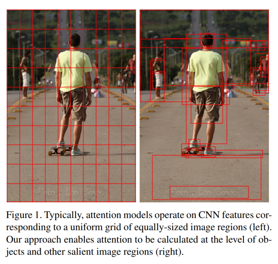

![image](https://user-images.githubusercontent.com/18450628/61817263-2683cd00-ae1c-11e9-971a-d3b531dbbd98.png)

## Combining the two

In this paper, the authors suggest using the bottom-up approach to compute the salient regions of the image the network should focus on using Faster-R-CNN. FRCNN is carefully pretrained on both imagenet and the Visual Genome dataset. It is then frozen and only used to generate bounding boxes of regions with high confidence of being of interest. The top-down approach is then used on the features obtained from the bottom-up approach. In order to "enhance" the FRCNN performance, they initialize their FRCNN with a ResNet-101 pre-trained on imagenet. They train their FRCNN on the Visual Genome dataset, adding attributes to the loss function that are available from the Visual Genome dataset, attributes such as color (black, white, gold etc.),  state (open, close, dark, bright, etc.). A sample of FRCNN outputs are shown in figure 2. It is important to stress that only the feature representations and not the actual outputs (i.e. not the labels) are used in their model.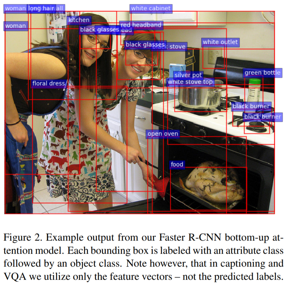

![image](https://user-images.githubusercontent.com/18450628/61817487-aca01380-ae1c-11e9-90fa-134033b95bb0.png)

## Caption Generation

Figure 3 provides a high-level overview of the model being used for caption generation for images. The image is first passed through FRCNN which produces a set of image features *V*. In their specific implementation, *V* consists of *k* vectors of size 1x2048. Their model consists of two LSTM blocks, one for attention and the other for language generation.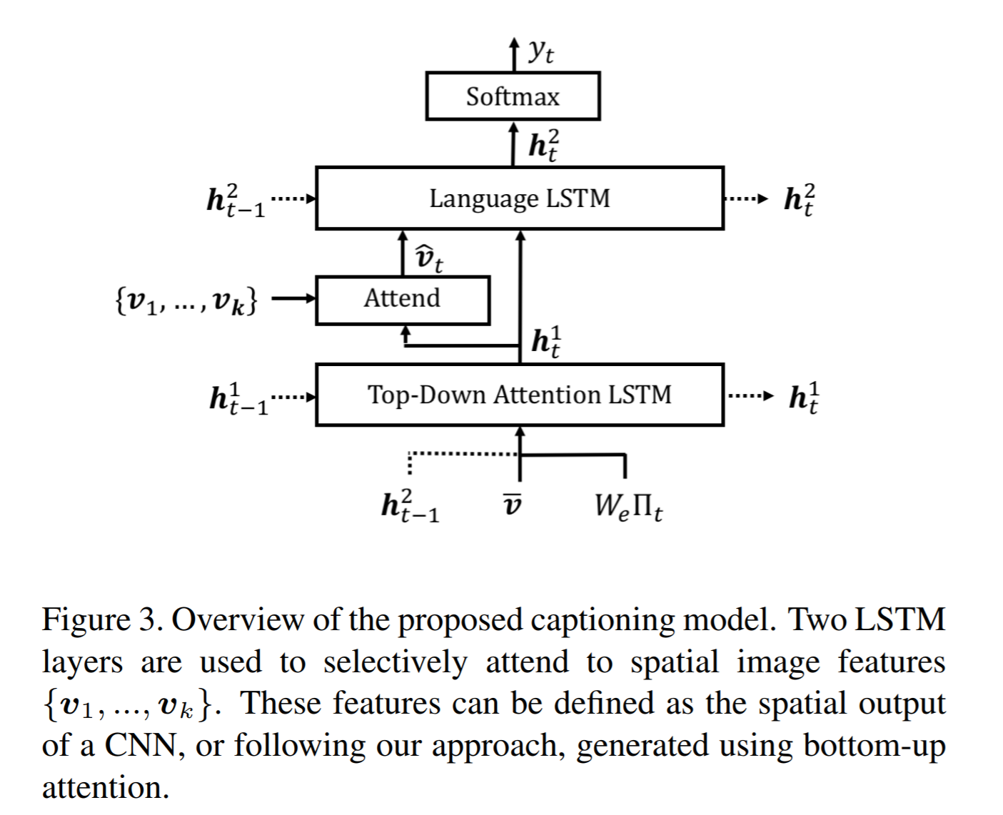

![image](https://user-images.githubusercontent.com/18450628/61818488-effb8180-ae1e-11e9-8ae4-14355115429a.png)

The first block of their model is a Top-Down Attention LSTM layer. It takes as input the mean-pooled features *V* , i.e. 1/k*sum(v_i), concatenated with the previous timestep's hidden representation of the language LSTM as well as the word embedding of the previously generated word. The word embedding is learned and not pretrained. 

The output of the first LSTM is used to compute the attention for each vector using an MLP and softmax: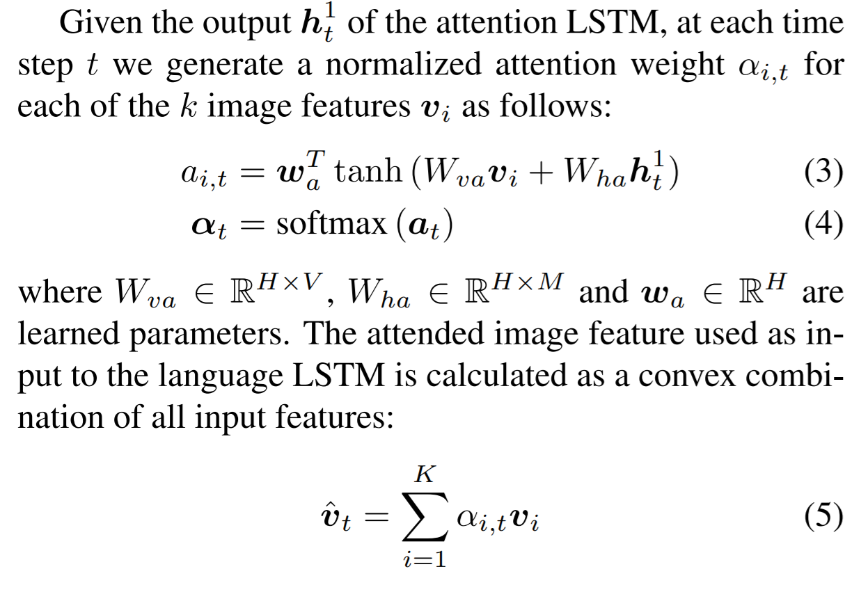

![image](https://user-images.githubusercontent.com/18450628/61819982-21298100-ae22-11e9-80a9-99640896413d.png)

The attention weighted image feature is then used as an input to the language LSTM model, concatenated with the output from the top-down Attention LSTM and a softmax is used to predict the next word in the sequence. The loss function seeks to minimize the cross-entropy of the generated sentence. 

## VQA Model

The VQA task differs to the image generation in that a text-based question accompanies an input image and the network must produce an answer. The VQA model proposed is different to that of the caption generation model previously described, however they both use the same bottom-up approach to generate the feature vectors of the image based on the FRCNN architecture. A high-level overview of the architecture for the VQA model is presented in Figure 4.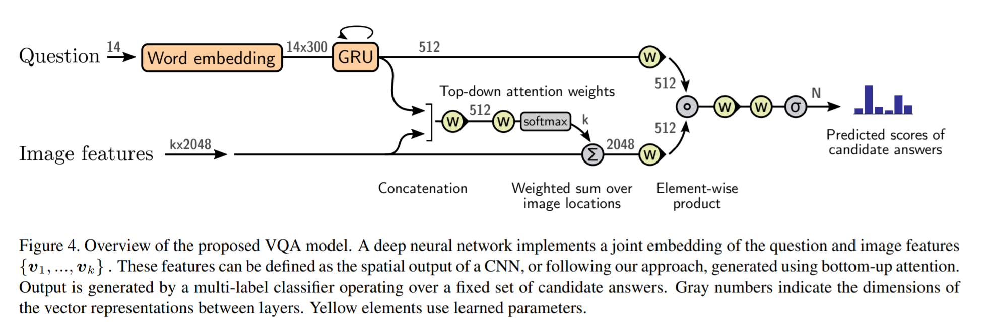

![image](https://user-images.githubusercontent.com/18450628/61821988-8da67f00-ae26-11e9-8456-3c9e5ec60787.png)

Each word from the question is converted to a learned word embedding which is used as input to a GRU. The number of words for each question is limited to 14 for computational efficiency. The output from the GRU is concatenated with each of the *k* image features, and attention weights are computed for each *k*th feature using an MLP and softmax, similar to what is done in the attention for caption generation. The weighted sum of the feature vectors is then passed through an linear layer such that its shape is compatible with the gru output, and the Hadamard product (element-wise product) is computed over the GRU output and attention-weighted image feature representation. Finally, a tanh non-linear activation is used. This results in a "gated tanh", which have been shown empirically to outperform both ReLU and tanh. Finally, a softmax probability distribution is generated at the output which selects a candidate answer among all possible candidate answers.

## Results and experiments

### Resnet Baseline

To demonstrate that their contribution of bottom-up mechanism actually improves on results, the authors use a ResNet trained on imagenet as a baseline for generating the image feature vectors (they resize the final CNN layers using bilinear interpolation when needed). They consistently obtain better results when using the bottom-up approach over the ResNet approach in both caption generation and VQA.

## MSCOCO

The authors demonstrate that they outperform all results on all metrics on the MSCOCO test server.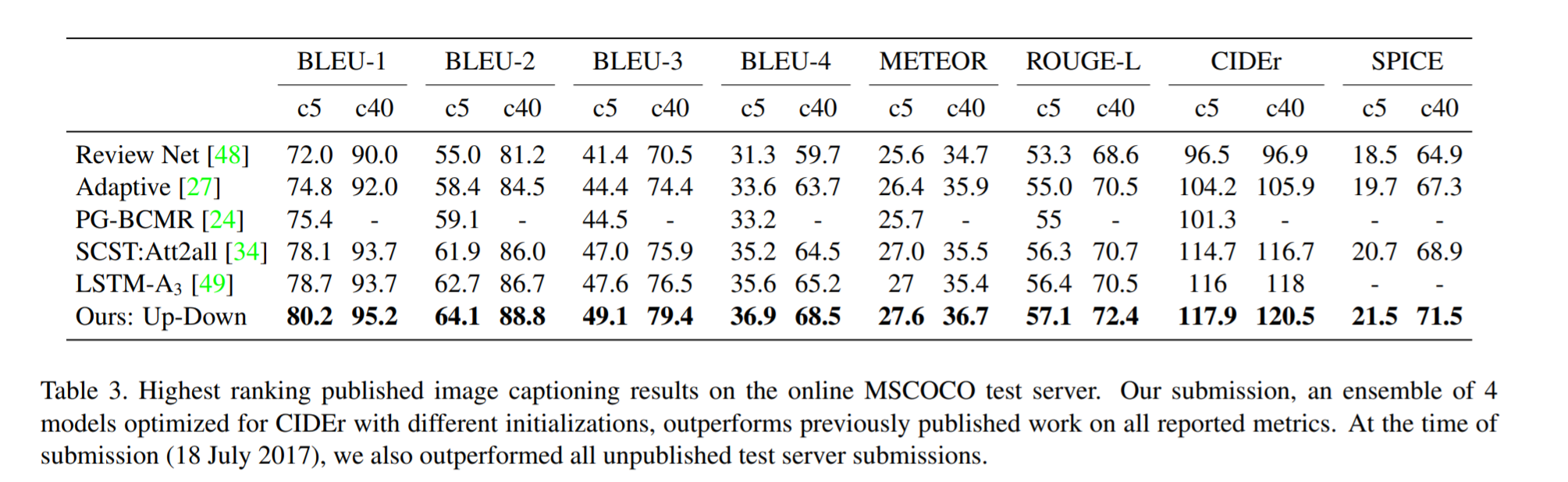

![image](https://user-images.githubusercontent.com/18450628/61824157-4f5f8e80-ae2b-11e9-8d90-657db453e26e.png)

They also show how using the bottom-up approach over ResNet consistently scores them higher on detecting instances of objects, attributes, relations, etc: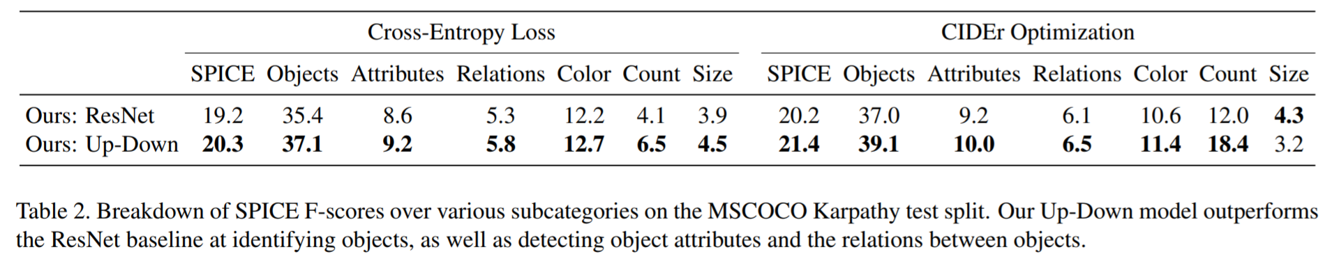

![image](https://user-images.githubusercontent.com/18450628/61824238-7fa72d00-ae2b-11e9-81b3-b5a7f80153f3.png)

The authors, like their predecessors, insist on demonstrating their network's frisbee ability: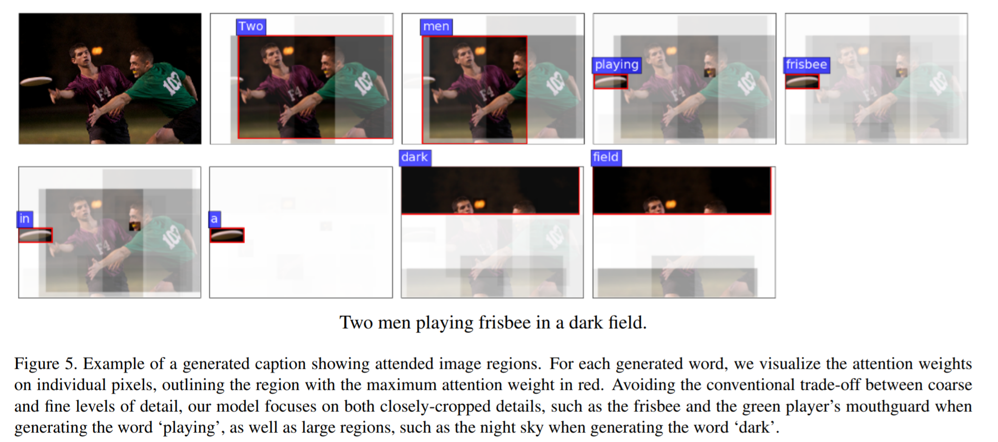

![image](https://user-images.githubusercontent.com/18450628/61824344-bed57e00-ae2b-11e9-87cd-597568587e1d.png)

## VQA Results

They also demonstrate that the addition of bottom-up attention improves results over a ResNet baseline.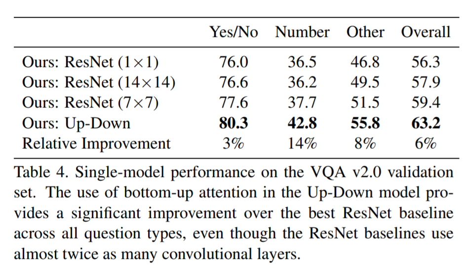 

![image](https://user-images.githubusercontent.com/18450628/61824500-28ee2300-ae2c-11e9-9016-2120a91917e4.png)

They also show that their model outperformed all other submissions on the VQA submission. They mention using an ensemble of 30 models for their submission.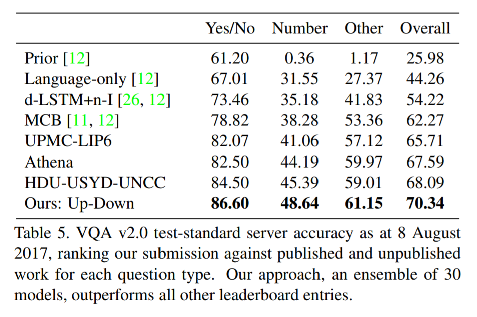 

![image](https://user-images.githubusercontent.com/18450628/61824634-83877f00-ae2c-11e9-8d84-9589e0ea2be2.png)


A sample image of what is attended in an image given a proper answer is shown in figure 6.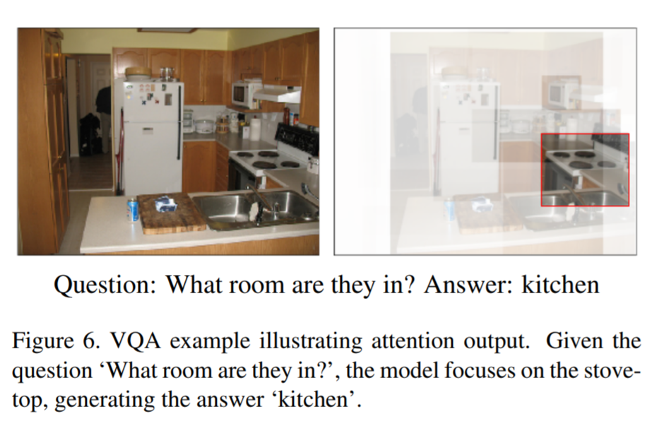

![image](https://user-images.githubusercontent.com/18450628/61824608-736f9f80-ae2c-11e9-9d4e-8cb6bd0a1a92.png)


# Comments

The authors introduce a new way to select portions of the image on which to focus attention. The idea is very original and came at a time when object detection was making significant progress (i.e. FRCNN).

A few comments:

* This method might not generalize well to other types of data. It requires pre-training on larger datasets (visual genome, imagenet, etc.) which consist of categories that overlap with both the MSCOCO and VQA datasets (i.e. cars, people, etc.). It would be interesting to see an end-to-end model that does not rely on pre-training on other similar datasets.

* No insight is given to the computational complexity nor to the inference time or training time. I imagine that FRCNN is resource intensive, and having to do a forward pass of FRCNN for every pass of the network must be a computational bottleneck. Not to mention that they ensembled 30 of them!

The paper designs some basic tests to compare saliency methods. It founds that some of the most popular methods are independent of model parameters and the data, meaning they are effectively useless.

## Methods compared

The paper compare the following methods: gradient explanation, gradient x input, integrated gradients, guided backprop, guided GradCam and SmoothGrad. They provide a refresher on those methods in the appendix.

All those methods can be put in the same framework. They require a classification model and an input (typically an image). The output of the method is an *explanation map* of the shape of the input where a higher value for a feature implies greater relevance in the decision of the model. 

## Metrics of comparison

The authors argue that visual inspection of the saliency maps can be misleading. They propose to compute the Spearman rank correlation, the structural similarity index (SSMI) and the Pearson correlation of the histogram of gradients. The authors point out that those metrics capture various notions of similarity, but it is an active area of research and those metrics are imperfect.

## First test: model parameters randomization

A saliency method must be dependent of model parameters, otherwise it cannot help us understand a model. In this test, the authors randomize the model parameters, layer per layer, starting from the top.

Surprisingly, methods such as guided backprop and guided gradcam are completely insensitive to model parameters, as illustrated on this Inception v3 trained on ImageNet:

![image](https://user-images.githubusercontent.com/8659132/61403152-b10b8000-a8a2-11e9-9f6a-cf1ed6a876cc.png)

Integrated gradients looks also dubious as the bird is still visible with a mostly fully randomized model, but the quantitative metrics reveal the difference is actually big between the two models.

## Second test: data randomization

It is well-known that randomly shuffling the labels of a dataset does not prevent a neural network from getting a high accuracy on the training set, though it does prevent generalization. The model is able to learn by either memorizing the data or finding spurious patterns. As a result, saliency maps obtained from such a network should have no clearly interpretable signal.

Here is the result for a ConvNet trained on MNIST and a shuffled MNIST:

![image](https://user-images.githubusercontent.com/8659132/61406757-7efe1c00-a8aa-11e9-9826-a859a373cb4f.png)

The results are very damning for most methods. Only gradients and GradCam are very different between both models, as confirmed by the low correlation.

## Discussion

- Even though some methods do no depend on model parameters and data, they might still depend on the architecture of the models, which could be of some use in some contexts.
- Methods that multiply the input with the gradient are dominated by the input.
- Complex saliency methods are just fancy edge detectors.
- Only gradient, smooth gradient and GradCam survives the sanity checks.

# Comments

- Why is their GradCam maps so ugly? They don't look like usual GradCam maps at all.
- Their tests are simple enough that it's hard to defend a method that doesn't pass them.
- The methods that are left are not very good either. They give fuzzy maps that are difficult to interpret.
- In the case of integrated gradients (IG), I'm not convinced this is sufficient to discard the method. IG requires a "baseline input" that represents the absence of features. In the case of images, people usually just set the image to 0, which is not at all the absence of a feature. The authors also use the "set the image to 0" strategy, and I'd say their tests are damning for this strategy, not for IG in general. I'd expect an estimation of the baseline such as done in [this paper](https://arxiv.org/abs/1702.04595) would be a fairer evaluation of IG.

Code: [GitHub](https://github.com/adebayoj/sanity_checks_saliency) (not available as of 17/07/19)

Li et al. propose an adversarial attack motivated by second-order optimization and uses input randomization as defense. Based on a Taylor expansion, the optimal adversarial perturbation should be aligned with the dominant eigenvector of the Hessian matrix of the loss. As the eigenvectors of the Hessian cannot be computed efficiently, the authors propose an approximation; this is mainly based on evaluating the gradient under Gaussian noise. The gradient is then normalized before taking a projected gradient step. As defense, the authors inject random noise on the input (clean example or adversarial example) and compute the average prediction over multiple iterations.

Also find this summary at [davidstutz.de](https://davidstutz.de/category/reading/).

Lecuyer et al. propose a defense against adversarial examples based on differential privacy. Their main insight is that a differential private algorithm is also robust to slight perturbations. In practice, this amounts to injecting noise in some layer (or on the image directly) and using Monte Carlo estimation for computing the expected prediction. The approach is compared to adversarial training against the Carlini+Wagner attack.

Also find this summary at [davidstutz.de](https://davidstutz.de/category/reading/).

Gowal et al. propose interval bound propagation to obtain certified robustness against adversarial examples. In particular, given a neural network consisting of linear layers and monotonic increasing activation functions, a set of allowed perturbations is propagated to obtain upper and lower bounds at each layer. These lead to bounds on the logits of the network; these are used to verify whether the network changes its prediction on the allowed perturbations. Specifically, Gowal et al. consider an $L_\infty$ ball around input examples; the initial bounds are, thus, $\underline{z}_0 = x - \epsilon$ and $\overline{z}_0 = x + \epsilon$. For each layer, the bounds are defined as

$\underline{z}_{k,i} = \min_{\underline{z}_{k – 1} \leq z_{k – 1} \leq \overline{z}_{k-1}} e_i^T h_k(z_{k – 1})$

and the analogous maximization problem for the upper bound; here, $h$ denotes the applied layer. For Linear layers and monotonic activation functions, this is easy to solve, as shown in the paper. Moreover, computing these bounds is very efficient, only needing roughly two times the computation of one forward pass. During training, a combination of a clean loss and adversarial loss is used:

$\kappa l(z_K, y) + (1 - \kappa) l(\hat{z}_K, y)$

where $z_K$ are the logits of the input $x$, and $\hat{z}_K$ are the adversarial logits computed as

$\hat{Z}_{K,y’} = \begin{cases} \overline{z}_{K,y’} & \text{if } y’ \neq y\\\underline{z}_{K,y} & \text{otherwise}\end{cases}$

Both $\epsilon$ and $\kappa$ are annealed during training. In experiments, it is shown that this method results in quite tight bounds on robustness.

Also find this summary at [davidstutz.de](https://davidstutz.de/category/reading/).

Zadeh et al. propose a layer similar to radial basis functions (RBFs) to increase a network’s robustness against adversarial examples by rejection. Based on a deep feature extractor, the RBF units compute

$d_k(x) = \|A_k^Tx + b_k\|_p^p$

with parameters $A$ and $b$. The decision rule remains unchanged, but the output does not resemble probabilities anymore. The full network, i.e., feature extractor and RBF layer, is trained using an adapted loss that resembles a max margin loss:

$J = \sum_i (d_{y_i}(x_i) + \sum_{j \neq y_i} \max(0, \lambda – d_j(x_i)))$

where $(x_i, y_i)$ is a training examples including label. The loss essentially minimizes the output corresponding to the true class while maximizing the output for all other classes up to a specified margin. Additionally, noise examples are injected during training. For these noise examples,

$\sum_j \max(0, \lambda – d_j(x))$

is maximized to enforce that these examples are treated as negatives in a rejection setting where samples not corresponding to the data distribution (or adversarial examples) can be rejected by the model. In experiments, the proposed method seems to be more robust against FGSM and iterative attacks (as evaluated on Foolbox).

Also find this summary at [davidstutz.de](https://davidstutz.de/category/reading/).

De Alfaro proposes a deep radial basis function (RBF) network to obtain robustness against adversarial examples. In contrast to “regular” RBF networks, which usually consist of only one hidden layer containing RBF units, de Alfaro proposes to stack multiple layers with RBF units. Specifically, a Gaussian unit utilizing the $L_\infty$ norm is used:

$\exp\left( - \max_i(u_i(x_i – w_i))^2\right)$

where $u_i$ and $w_i$ are parameters and $x_i$ are the inputs to the unit – so the network inputs or the outputs of the previous hidden layer. This unit can be understood as computing a soft AND operation; therefore, an alternative OR operation

$1 - \exp\left( - \max_i(u_i(x_i – w_i))^2\right)$

is used as well. These two units are used alternatingly in hidden layers in the conducted experiments. Based on these units, de Alfaro argues that the model is less sensitive to adversarial examples, compared to linear operations as commonly used in ReLU networks.

For training a deep RBF-network, pseudo gradients are used for both the maximum operation and the exponential function. This is done for simplifying training; I refer to the paper for details.

In their experiments, on MNIST, a multi-layer perceptron with the proposed RBF units is used. The network consists of 512 AND units, 512 OR units, 512 AND units and finally 10 OR units. Robustness against FGSM and I-FGSM as well as PGD attacks seems to improve. However, the used PGD attack seems to be weaker than usually, it does not manage to reduce adversarial accuracy of a normal networks to near-zero.

Also find this summary at [davidstutz.de](https://davidstutz.de/category/reading/).

Morcos et al. study the influence of ablating single units as a proxy to generalization performance. On Cifar10, for example, a 11-layer convolutional network is trained on the clean dataset, as well as on versions of Cifar10 where a fraction of $p$ samples have corrupted labels. In the latter cases, the network is forced to memorize examples, as there is no inherent structure in the labels assignment. Then, it is experimentally shown that these memorizing networks are less robust to setting whole feature maps to zero, i.e., ablating them. This is shown in Figure 1. Based on this result, the authors argue that the area under this ablation curve (AUC) can be used as proxy for generalization performance. For example, early stopping or hyper-parameter selection can be done based on this AUC value. Furthermore, they show that batch normalization discourages networks to rely on these so-called single-directions, i.e., single units or feature maps. Specifically, batch normalization seems to favor units holding information about multiple classes/concepts.


https://i.imgur.com/h2JwLUF.png
Figure 1: Classification accuracy (y-axis) over the number of units that are ablated (x-axis) for networks trained on Cifar10 with various degrees of corrupted labels. The same experiments (left and right) for MNIST and ImageNet.

Also find this summary at [davidstutz.de](https://davidstutz.de/category/reading/).

Xie et al. propose to improve the transferability of adversarial examples by computing them based on transformed input images. In particular, they adapt I-FGSM such that, in each iteration, the update is computed on a transformed version of the current image with probability $p$. When, at the same time attacking an ensemble of networks, this is shown to improve transferability.

Also find this summary at [davidstutz.de](https://davidstutz.de/category/reading/).

Liu et al. propose adversarial attacks on physical parameters of images, which can be manipulated efficiently through differentiable renderer. In particular, they propose adversarial lighting and adversarial geometry; in both cases, an image is assumed to be a function of lighting and geometry, generated by a differentiable renderer. By directly manipulating these latent variables, more realistic looking adversarial examples can be generated for synthetic images as shown in Figure 1.

https://i.imgur.com/uh2pj9w.png
Figure 1: Comparison of the proposed attack with known attacks applied to large perturbations, $L_\infty \approx 0.82$.

Also find this summary at [davidstutz.de](https://davidstutz.de/category/reading/).

Zhou et al. study transferability of adversarial examples against ensembles of randomly perturbed networks. Specifically, they consider randomly perturbing the weights using Gaussian additive noise. Using an ensemble of these perturbed networks, the authors show that transferability of adversarial examples decreases significantly. However, the authors do not consider adapting their attack to this defense scenario.

Also find this summary at [davidstutz.de](https://davidstutz.de/category/reading/).

Thang and Evanse propose cost-sensitive certified robustness where different adversarial examples can be weighted based on their actual impact for the application. Specifically, they consider the certified robustness formulation (and the corresponding training scheme) by Wong and Kolter. This formulation is extended by acknowledging that different adversarial examples have different impact for specific applications; this is formulized through a cost matrix which quantifies which source-target label combinations of adversarial examples are actually harmful. Based on this cost matrix, cost-sensitive certified robustness as well as the corresponding training scheme is proposed and evaluated in experiments.

Also find this summary at [davidstutz.de](https://davidstutz.de/category/reading/).

Ilyas et al. propose three query-efficient black-box adversarial example attacks using distribution-based gradient estimation. In particular, their simplest attacks involves estimating the gradient locally using a search distribution:

$ \nabla_x \mathbb{E}_{\pi(\theta|x)} [F(\theta)] = \mathbb{E}_{\pi(\theta|x)} [F(\theta) \nabla_x \log(\pi(\theta|x))]$

where $F(\cdot)$ is a loss function – e.g., using the cross-entropy loss which is maximized to obtain an adversarial example. The above equation, using a Gaussian noise search distribution leads to a simple approximator for the gradient:

$\nabla \mathbb{E}[F(\theta)] = \frac{1}{\sigma n} \sum_{i = 1}^n \delta_i F(\theta + \sigma \delta_i)$

where $\sigma$ is the search variance and $\delta_i$ are sampled from a unit Gaussian. This scheme can then be applied as part of the projected gradient descent white-box attacks to obtain adversarial examples.

The above attack assumes that the black-box network provides probability outputs in order to compute the loss $F$. In the remainder of the paper, the authors also generalize this approach to the label-only case, where the network only provides the top $k$ labels for each input. In experiments, the attacks is shown to be effective while rarely requiring more than $50$k queries on ImageNet.

Also find this summary at [davidstutz.de](https://davidstutz.de/category/reading/).

Demontis et al. study transferability of adversarial examples and data poisening attacks in the light of the targeted models gradients. In particular, they experimentally validate the following hypotheses: First, susceptibility to these attacks depends on the size of the model’s gradients; the higher the gradient, the smaller is the perturbation needed to increase the loss. Second, the size of the gradient depends on regularization. And third, the cosine between the target model’s gradients and the surrogate model’s gradients (trained to compute transferable attacks) influences vulnerability. These insights hold for both evasion and poisening attacks and are motivated by a simple linear Taylor expansion of the target model’s loss.

Also find this summary at [davidstutz.de](https://davidstutz.de/category/reading/).

Khoury and Hadfield-Menell provide two important theoretical insights regarding adversarial robustness: it is impossible to be robust in terms of all norms, and adversarial training is sample inefficient. Specifically, they study robustness in relation to the problem’s codimension, i.e., the difference between the dimensionality of the embedding space (e.g., image space) and the dimensionality of the manifold (where the data is assumed to actually live on). Then, adversarial training is shown to be sample inefficient in high codimensions.

Also find this summary at [davidstutz.de](https://davidstutz.de/category/reading/).

Grosse et al. show that Gaussian Processes allow to reject some adversarial examples based on their confidence and uncertainty; however, attacks maximizing confidence and minimizing uncertainty are still successful. While some state-of-the-art adversarial examples seem to result in significantly different confidence and uncertainty estimates compared to benign examples, Gaussian Processes can still be fooled through particularly crafted adversarial examples. To this end, the confidence is explicitly maximized and, additionally, the uncertainty is constrained to not be larger than the uncertainty of the corresponding benign test example. In experiments, this attack is shown to successfully fool Gaussian Processes while resulting in imperceptible perturbations.

Also find this summary at [davidstutz.de](https://davidstutz.de/category/reading/).

Carlini et al. propose several attacks to extract secrets form trained black-box models. Additionally, they show that state-of-the-art neural networks memorize secrets early during training. Particularly on the Penn treebank, after inserting a secret of specific format, the authors validate that the secret can be identified based on the models output probabilities (i.e., black-box access). Several metrics based on the log-perplexity of the secret show that secrets are memorized early during training and memorization happens for all popular architectures and training strategies; additionally, memorization also works for multiple secrets. Furthermore, the authors propose several attacks to extract secrets, most notably through shortest path search. Here, starting with an empty secret, the characters of the secret are identified sequentially in order to minimize log-perplexity. Using this attack, secrets such as credit card numbers are extractable from popular mail datasets.

Also find this summary at [davidstutz.de](https://davidstutz.de/category/reading/).

Pérolat et al. propose a game-theoretic variant of adversarial training on universal adversarial perturbations. In particular, in each training iteration, the model is trained for a specific number of iterations on the current training set. Afterwards, a universal perturbation is found (and the corresponding test images) that fools the network. The found adversarial examples are added to the training set. In the next iteration, the network is trained on the new training set which includes adversarial examples. Overall, this leads to a network being trained on a sequence of universal adversarial perturbations corresponding to earlier versions of that network.

Also find this summary at [davidstutz.de](https://davidstutz.de/category/reading/).

Shafahi et al. discuss fundamental limits of adversarial robustness, showing that adversarial examples are – to some extent – inevitable. Specifically, for the unit sphere, the unit cube as well as for different attacks (e.g., sparse attacks and dense attacks), the authors show that adversarial examples likely exist. The provided theoretical arguments also provide some insights on which problems are more (or less) robust. For example, more concentrated class distributions seem to be more robust by construction. Overall, these insights lead the authors to several interesting conclusions:  First, the results are likely to extent to datasets which actually live on low-dimensional manifolds of the unit sphere/cube. Second, it needs to be differentiated between the existence adversarial examples and our ability to compute them efficiently. Making it harder to compute adversarial examples might, thus, be a valid defense mechanism. And third, the results suggest that lower-dimensional data might be less susceptible to adversarial examples.

Also find this summary at [davidstutz.de](https://davidstutz.de/category/reading/).

Shafahi et al. propose universal adversarial training, meaning training on universal adversarial examples. In contrast to regular adversarial examples, universal ones represent perturbations that cause a network to mis-classify many test images. In contrast to regular adversarial training, where several additional iterations are required on each batch of images, universal adversarial training only needs one additional forward/backward pass on each batch. The obtained perturbations for each batch are accumulated in a universal adversarial examples. This makes adversarial training more efficient, however reduces robustness significantly.

Also find this summary at [davidstutz.de](https://davidstutz.de/category/reading/).

Lamb et al. introduce fortified networks with denoising auto encoders as hidden layers. These denoising auto encoders are meant to learn the manifold of hidden representations, project adversarial input back to the manifold and improve robustness. The main idea is illustrated in Figure 1. The denoising auto encoders can be added at any layer and are trained jointly with the classification network – either on the original input, or on adversarial examples as done in adversarial training.

https://i.imgur.com/5vaZrVk.png
Figure 1: Illustration of a fortified layer, i.e., a hidden layer that is reconstructed through a denoising auto encoder as defense mechanism. The denoising auto encoders are trained jointly with the network.

In experiments, they show that the proposed defense mechanism improves robustness on MNIST and CIFAR, compared to adversarial training and other baselines. The improvements are, however, very marginal. Especially, as the proposed method imposes an additional overhead (in addition to adversarial training).

Also find this summary at [davidstutz.de](https://davidstutz.de/category/reading/).

Schott et al. propose an analysis-by-synthetis approach for adversarially robust MNIST classification. In particular, as illustrated in Figure 1, class-conditional variational auto-encoders (i.e., one variational auto-encoder per class) are learned. The respective recognition models, i.e., encoders, are discarded. For classification, the optimization problem

$l_y^*(x) = \max_z \log p(x|z) - \text{KL}(\mathcal{N}(z, \sigma I)|\mathcal{N}(0,1))$

is solved for each class $z$. Here, $p(x|z)$ represents the learned generative model. The optimization problem leads a latent code $z$ corresponding to the best reconstruction of the input. The corresponding likelihood can be used for classificaiton using Bayes’ theorem. The obtained posteriors $p(y|x)$ are then scaled using a modified softmax (see paper) to obtain the final decision. (Additionally, input binarization is used as defense.)

https://i.imgur.com/ignvoHQ.png
Figure 1: The proposed analysis by synthesis approach to MNIST classification. The depicted generators are taken from class-specific variational auto-encoders.

In addition to the proposed defense, Schott et al. also derive lower and upper bounds on the robustness of the classification procedure. These bounds can be derived from the optimization problem above, see the paper for details.

In experiments, they show that their defense outperforms state-of-the-art adversarial training and allows to estimate tight bounds. In addition, the method is robust against distal adversarial examples and the adversarial examples look more meaningful, see Figure 2.

https://i.imgur.com/uxGzzg1.png
Figure 2: Adversarial examples for the proposed “ABS” method, its binary variant and related work.

Also find this summary at [davidstutz.de](https://davidstutz.de/category/reading/).

Galloway et al. provide a theoretical and experimental discussion of adversarial training and weight decay with respect to robustness as well as generalization. In the following I want to try and highlight the most important findings based on their discussion of linear logistic regression. Considering the softplus loss $\mathcal{L}(z) = \log(1 + e^{-z})$, the learning problem takes the form:

$\min_w \mathbb{E}_{x,y \sim p_{data}} [\mathcal{L}(y(w^Tx + b)]$

where $y \in \{-1,1\}$. This optimization problem is also illustrated in Figure 1 (top). Now considering $L_2$ weight decay can also be seen to be equivalent to scaling the softplus loss. In particular, Galloway et al. Argue that $w^Tx + b = \|w\|_2 d(x)$ where $d(x)$ is the (signed) Euclidean distance to the decision boundary. (This follows directly from the fact that $d(x) = \frac{w^Tx +b}{\|w\|w_2}$.) Then, the problem can be rewritten as

$\min_w \mathbb{E}_{x,y \sim p_{data}} [\mathcal{L}(yd(x) \|w\|_2)]$

This can be understood as a scaled version of the softplus loss; adding a $L_2$ weight decay term basically controls the level of scaling. This is illustrated in Figure 1 (middle) for different levels of scaling. Finally, adversarial training means training on the worst-case example for a given $\epsilon$. In practice, for the linear logistic regression model, this results in training on $x - \epsilon y \frac{w}{\|w\|_2}$ - which can easily be understood when considering that the attacker can cause the most disturbance when changing the samples in the direction of $-w$ for label $1$. Then,

$y (w^T(x - \epsilon y \frac{w}{\|w\|_2}) + b) = y(w^Tx + b) - \epsilon \|w\|_2 = \|w\|_2 (yd(x) - \epsilon)$,

which results in a shift of the data by $\epsilon$ - as illustrated in Figure 1 (bottom). Overall, show that weight decay acts as scaling the objective and adversarial training acts as shifting the data (or equivalently the objective).

In the non-linear case, decaying weights is argued to be equivalent to decaying the logits. Effectively, this results in a temperature parameter for the softmax function resulting in smoother probability distributions. Similarly, adversarial training (in a first-order approximation) can be understood as effectively reducing the probability attributed to the correct class. Here, again, weight decay results in a scaling effect and adversarial training in a shifting effect. In conclusion, adversarial training is argued to be only effective with small perturbation sizes (i.e., if the shift is not too large), weil weight decay is also beneficial for generalization. However, from reading the paper, it is unclear what the actual recommendation on both methods is.

In the experimental section, the authors focus on two models, a wide residual network and a very constrained 4-layer convolutional neural network. Here, their discussion shifts slightly to the complexity of the employed model. While not stated very explicitly, one of the take-aways is that the simpler model might be more robust, especially for fooling images.

https://i.imgur.com/FKT3a2O.png
https://i.imgur.com/wWwFKqn.png
https://i.imgur.com/oaTfqHJ.png
Figure 1: Illustration of the linear logistic regression argument. Top: illustration of linear logistic regression where $\xi$ is the loss $\mathcal{L}$, middle: illustration of the impact of weight decay/scaling, bottom: illustration of the impact of shift for adversarial training.

Also find this summary at [davidstutz.de](https://davidstutz.de/category/reading/).

What is stopping us from applying meta-learning to new tasks? Where do the tasks come from? Designing task distribution is laborious. We should automatically learn tasks!

Unsupervised Learning via Meta-Learning: The idea is to use a distance metric in an out-of-the-box unsupervised embedding space created by BiGAN/ALI or DeepCluster to construct tasks in an unsupervised way. If you cluster points to randomly define classes (e.g. random k-means) you can then sample tasks of 2 or 3 classes and use them to train a model.

Where does the extra information come from? The metric space used for k-means asserts specific distances. The intuition why this works is that it is useful model initialization for downstream tasks.

This summary was written with the help of Chelsea Finn.

In terms of model based RL, learning dynamics models is imperfect, which often leads to the learned policy overfitting to the learned dynamics model, doing well in the learned simulator but not in the real world.

Key solution idea: No need to try to learn one accurate simulator. We can learn an ensemble of models that together will sufficiently represent the space. If we learn an ensemble of models (to be used as many learned simulators) we can denoise estimates of performance. In a meta-learning sense these simulations become the tasks. The real world is then just yet another task, to which the policy could adapt quickly.  One experimental observation is that at the start of training there is a lot of variation between learned simulators, and then the simulations come together over training, which might also point to this approach providing improved exploration.

This summary was written with the help of Pieter Abbeel.

In the area of explaining model predictions over images, there are two main strains of technique: methods that look for pixels that have the highest gradient effect on the output class, and assign those as the “reason” for the class, and approaches that ask which pixel regions are most responsible for a given classification, in the sense that the classification would change the most if they were substituted with some uninformative reference value. 

The tricky thing about the second class of methods is that you need to decide what to use as your uninformative fill-in value. It’s easy enough to conceptually pose the problem of “what would our model predict if it couldn’t see this region of pixels,” but as a practical matter, these models take in full images, and you have to put *something* to give the classifier in a region, if you’re testing what the score would be if you removed the information contained in the pixels in that region. What should you fill in instead? The simplest answers are things like “zeros”, or “a constant value” or “white noise”. But all of these are very off-distribution for the model; it wouldn’t have typically seen images that resemble white noise, or all zeros, or all a single value. So if you measure the change in your model score from an off-distribution baseline to your existing pixels, you may not be getting the marginal value of the pixels, so much as the marginal disutility of having something so different from what the model has previously seen. There are other, somewhat more sensible approaches, like blurring out the areas around the pixel region of interest, but these experience less intense forms of the same issue. 

This paper proposes instead, using generative models to fill in the regions conditioned on the surrounding pixels, and use that as a reference. The notion here is that a conditioned generative model, like a GAN or VAE, can take into account the surrounding pixels, and “imagine” a fill-in that flows smoothly from the surrounding pixels, and looks generally like an image, but which doesn’t contain the information from the pixels in the region being tested, since it wasn’t conditioned on that. 

https://i.imgur.com/2fKnY0M.png

Using this approach, the authors run two types of test: one where they optimize to find the smallest region they can remove from the image, and have it switch class (Smallest Deletion Region, or SDR), and also the smallest informative region that can be added to an otherwise uninformative image, and have the model predict the class connected to that region. They find that regions calculated using their generative model fill in, and specifically with GANs, find a smaller and more compact pixel region as their explanation for the prediction, which is consistent with both human intuitions and also with a higher qualitative sensibleness of the explanations found. 

This was definitely one of the more conceptually nuanced and complicated papers I’ve read recently, and I’ve only got about 60% confidence that I fully grasp all of its intuitions. However, I’m going to try to collect together what I did understand. 

There is a lot of research into generative models of text or image sequences, and some amount of research into building “models” in the reinforcement learning sense, where your model can predict future observations given current observations and your action. There’s an important underlying distinction here between model-based RL (where you learn a model of how the world evolves, and use that to optimize reward) and model-free RL (where you leave don’t bother explicitly learning a world model, and just directly try to optimize rewards)  However, this paper identifies a few limitations of this research. 

1) It’s largely focused on predicting observations, rather than predicting *state*. State is a bit of a fuzzy concept, and corresponds to, roughly, “the true underlying state of the game”. An example I like to use is a game where you walk in one door, and right next to it is a second door, which requires you to traverse the space and find rewards and a key before you can open. Now, imagine that the observation of your agent is it looking at the door. If the game doesn’t have any on-screen representation of the fact that you’ve found the key, it won’t be present in your observations, and you’ll observe the same thing at the point you have just entered and once you found the key. However, the state of the game at these two points will be quite different, in that in the latter case, your next states might be “opening the door” rather than “going to collect rewards”. Scenarios like this are referred to broadly as Partially Observable games or environments. This paper wants to build a model of how the game evolves into the future, but it wants to build a model of *state-to-state* evolution, rather than observation-to-observation evolution, since observations are typically both higher-dimensionality and also more noisy/less informative. 

2) Past research has typically focused on predicting each next-step observation, rather than teaching models to be able to directly predict a state many steps in the future, without having to roll out the entire sequence of intermediate predictions.  This is arguably quite valuable for making models that can predict the long term consequences of their decision 

This paper approaches that with an approach inspired by the Temporal Difference framework used in much of RL, in which you update your past estimate of future rewards by forcing it to be consistent with the actual observed rewards you encounter in the future. Except, in this model, we sample two a state (z1) and then a state some distance into the future (z2), and try to make our backwards-looking prediction of the state at time 1, taking into account observations that happened in between, match what our prediction was with only the information at time one. 

An important mechanistic nuance here is the idea of a “belief state”, something that captures all of your knowledge about game history up to a certain point. We can then directly sample a state Zt given the belief state Bt at that point. This isn’t actually possible with a model where we predict a state at time T given the state at time T-1, because the state at time Z-1 is itself a sample, and so in order to get a full distribution of Zt, you have to sample Zt over the distribution of Zt-1, and in order to get the distribution of Zt-1 you have to sample over the distribution of Zt-2, and so on and so on. Instead, we have a separate non-state variable, Bt that is created conditional on all our past observations (through a RNN). 

https://i.imgur.com/N0Al42r.png

All said and done, the mechanics of this model look like: 
1) Pick two points along the sequence trajectory
2) Calculate the belief state at each point, and, from that, construct a distribution over states at each timestep using p(z|b) 
3) Have an additional model that predicts z1 given z2, b1, and b2 (that is, the future beliefs and states), and push the distribution over z1 from this model to be close to the distribution over z1 given only the information available at time t1
4) Have a model that predicts Z2 given Z1 and the time interval ahead that we’re jumping, and try to have this model be predictive/have high likelihood over the data 
5) And, have a model that predicts an observation at time T2 given the state Z2, and train that so that we can convert our way back to an observation, given a state 

They mostly test it on fairly simple environments, but it’s an interesting idea, and I’d be curious to see other people develop it in future. 

(A strange aspect of this model is that, as far as I can tell, it’s non-interventionist, in that we’re not actually conditioning over agent action, or trying to learn a policy for an agent. This is purely trying to learn the long term transitions between states) 

Unsupervised representation learning is a funny thing: our aspiration in learning representations from data is typically that they’ll be useful for future tasks, but, since we (by definition) don’t have access to labels, our approach has historically been to define heuristics, such as representing the data distribution in a low-dimensional space, and hope that those heuristics translate to useful learned representations. And, to a fair extent, they have. However, this paper’s goal is to attach this problem more directly, by explicitly meta-learning an unsupervised update rule so that performs well in future tasks. They do this by: 

https://i.imgur.com/EEkpW9g.png

1) Defining a parametrized weight update function, to slot into the role that Stochastic Gradient Descent on a label-defined loss function would play in a supervised network. This function calculates a “hidden state”, is defined for each neuron in each layer, and takes in the pre and post-nonlinearity activations for that batch, the hidden state of the next layer, and a set of learned per-layer “backwards weights”. The weight update for that neuron is then calculated using the current hidden state, the last batch's hidden state, and the current value of the weight. In the traditional way of people in this field who want to define some generic function, they instantiate these functions as a MLP. 

2) Using that update rule on the data from a new task, taking the representing resulting from applying the update rule, and using it in a linear regression with a small number of samples. The generalization performance from this k-shot regression, taken in expectation over multiple tasks, acts as our meta training objective. By back-propagating from this objective, to the weight values of the representation, and from there to the parameters of the optimization step, they incentivize their updater to learn representations that are useful across some distribution of tasks. 


A slightly weird thing about this paper is that they train on image datasets, but shuffle the pixels and use a fully connected network rather than a conv net. I presume this has to do with the complexities of defining a weight update rule for a convolution, but it does make it harder to meaningfully compare with other image-based unsupervised systems, which are typically done using convolution. An interesting thing they note is that, early in meta-training on images, their update rules generalize fairly well to text data. However, later in training the update rules seem to have specialized to images, and generalize more poorly to images. 

This paper out of DeepMind used a Google StreetView dataset and set out to train a network capable of navigating to a given goal destination, without knowing where it was on any birds-eye map, and with its only input being photographic viewpoint images of its current location and orientation. This was done through a framework of reinforcement learning, where the model is conditioned on a representation of its goal, and given the image features of its current view of the world, and has to take actions like “turn left,” “turn sharply left”, “go forward”, etc, in order to navigate. Rather than lat-long, goals are specified in city-specific ways, in terms of the distance between the goal position and a reference set of landmarks. I don’t entirely understand the motivation behind this approach; the authors say it’s more scalable, but it wasn’t obvious to me why that would be the case. 

https://i.imgur.com/V3UATsK.png

- The authors construct different architectures that combine these two fundamental pieces of input data - current image and the goal you’re trying to reach - in different ways. 
In the simplest model, called GoalNav, there’s a single LSTM that combines the goal information with the output of a convolutional encoder processing images of your current viewpoint.
- In the next most complex, CityNav, there are two LSTMs: one for processing your goal, and the other for combining the output of the goal network with your convolutional inputs, in order to decide on an action. Notionally, this separation of tasks corresponds to “figure out what absolute to go in, given your goal”, and “figure out how to go in that absolute direction from where you are now”. As a way to support training, the goal network is trained with an auxiliary loss function where it needs to predict how far its current orientation is from North. Note that this does pass some amount of information about current location into the model (since the network gets to know its actual orientation relative to true north), but this is only available during training, with the hope that the model will have gotten good enough at predicting orientation to perform well.  
- The final model, similar to above, is called MultiCityNav, and is explicitly designed for transfer learning. Instead of training multiple cities on a single shared network, only the convolutional encoder and policy network (the “how do I go in the absolute direction needed to reach my goal” parts) are shared between cities, and the goal processing LSTM (the “which direction should I be going in” part) is re-trained per city. This is designed to allow for transfer in the parts of learning you would expect to generalize, but allow the network to learn a city-specific approach for converting between goal specifications (in terms of city landmarks) and direction. 

In order to get over the fact that reward in this setting is very sparse (i.e. you only get reward when you reach the goal), the authors (1) train in a curriculum fashion, starting with tasks very nearby the model’s starting point, and gradually getting longer, and (2) add a small amount of reward shaping, where you get rewarded for moving in the direction of the goal, but only if you’re within 200m of it. This last is a bit of a concession on the realism front, and the authors say as much, but it’s just quite hard to train RL with purely dense rewards, and it makes sense that reward shaping would help here. 

Ultimately, they were able to get performance (in terms of goal-reaching rewards) around ¾ as strong as an Oracle model, who had access to the full map and could calculate the true shortest path.

The paper discusses neural module network trees (NMN-trees). Here modules are composed in a tree structure to answer a question/task and modules are trained in different configurations to ensure they learn more core concepts and can generalize.

Longer summary:

How to perform systematic generalization? First we need to ask how
good current models are at understanding language. Adversarial
examples show how fragile these models can be. This leads us to
conclude that systematic generalization is an issue that requires
specific attention.

Maybe we should rethink the modeling assumptions being made. We can
think that samples can come from different data domains but are
generated by some set of shared rules. If we correctly learned these
rules then domain shift in the test data would not hurt model
performance. Currently we can construct an experiment to introduce
systematic bias in the data which causes the performance to suffer.
From this experiment we can start to determine what the issue is.

A recent new idea is to force a model to have more independent units
is neural module network trees (NMN-trees). Here modules are composed
in a tree structure to answer a question/task and modules are trained
in different configurations to ensure they learn more core concepts
and can generalize.

[I do occasionally wonder if people will look back on the “Is All You Need” with genuine confusion in a few years. “Really…all you need?”]

This paper merges the ideas of curiosity-based learning and hierarchical reinforcement learning, to propose an architecture for learning distinctive skills based solely on an incentive to make those skills distinguishable from one another and relatively internally random, rather than because they’re directly useful in achieving some reward. 

The notion of hierarchical reinforcement learning is that, instead of learning a single joint policy, we learn some discrete number of subpolicies, and then treat the distribution over those subpolicies as you would a distribution over actions in a baseline RL policy. In order to achieve a reward, a model jointly optimizes the action distribution of the subpolicies, and also the distribution over subpolicies. One issue with this approach, which is raised by this paper (though I don’t really have strong enough domain background here to know how much of a problem this is in practice) is that this joint optimization process means that, early in the process, we choose subpolicies that are doing the best, and sample more from and thus improve those. This “early exploitation” problem (in the explore vs exploit frame) means that we might not learn skills that would be valuable to know later on, but that don’t give us any reward until we’ve developed them further. 

To address this, this paper proposes DIAYN, an algorithm which (1) samples discrete latent skill vectors according to a uniform, high-entropy prior, rather than according to how useful we think they are now, and (2) doesn’t even have a direct notion of usefulness, but instead incentivizes shaping of skills to be more distinct from one another, in terms of the states that are visited by each skill’s policy. The network then learns policies conditioned on each skill vector, and at each point operates according to whichever has been sampled. This idea of distinctiveness is encapsulated by saying “we want to have high mutual information between the states visited by a skill, and the discrete ID of that skill,” or, in more practical terms, “we want to be able to train a discriminator to do a good job predicting which skill we’re sampling from, based on the states it sees. (I swear, every time I read a paper where someone uses mutual information these days, it’s actually a discriminator under the hood).

https://i.imgur.com/2a378Bo.png

This incentivizes the model to take actions associated with each skill that will get it to states that are unlikely to occur in any of the existing skills. Depending on what set of observations you give the discriminator to work with, you can shape what axes your skills are incentivized to vary on; if you try to discriminate skills based solely on an agent’s center of mass, you’ll end up with policies that vary their center of mass more wildly. The paper shows that, at least on simple environments, agents can learn distinctive clusters of skills based on this objective. 

An interesting analogy here is to unsupervised pretraining of e.g. large language models and other similar settings, where we first train a model without (potentially costly) explicit reward, and this gives us a starting point set of representations that allow us to reach good performance more quickly once we start training on supervised reward signal. There is some evidence that this pretraining effect could be captured by this kind of purely-exploratory approach, as suggested by experiments done to take the learned skills or subpolicies, hold them fixed, and train a meta-controller to pick subpolicies according to an external reward, where the “pretrained” policy reaches high reward more quickly. 

The paper looks at approaches to predicting individual survival time distributions (isd). The motivation is shown in the figure below. Between two patients the survival time varies greatly so we should be able to predict a distribution like the red curve.

https://i.imgur.com/2r9JvUp.png

The paper studies the following methods: 
 - class-based survival curves Kaplan-Meier [31]
 - Kalbfleisch-Prentice extension of the Cox (cox-kp) [29]
 - Accelerated Failure Time (aft) model [29]
 - Random Survival Forest model with Kaplan-Meier extensions (rsf-km)
 - elastic net Cox (coxen-kp) [55] 
 - Multi-task Logistic Regression (mtlr) [57]

Looking at the predictions of these methods side by side we can observe some systematic differences between the methods:
https://i.imgur.com/vJoCL4a.png

The paper presents a "D-Calibration" metric (distributional calibration) which represents of the method answers this question:

    Should the patient believe the predictions implied by the survival curve?


https://i.imgur.com/MX8CbZ7.png

Papernot and McDaniel introduce deep k-nearest neighbors where nearest neighbors are found at each intermediate layer in order to improve interpretbaility and robustness. Personally, I really appreciated reading this paper; thus, I will not only discuss the actually proposed method but also highlight some ideas from their thorough survey and experimental results.

First, Papernot and McDaniel provide a quite thorough survey of relevant work in three disciplines: confidence, interpretability and robustness. To the best of my knowledge, this is one of few papers that explicitly make the connection of these three disciplines. Especially the work on confidence is interesting in the light of robustness as Papernot and McDaniel also frequently distinguish between in-distribution and out-distribution samples. Here, it is commonly known that deep neural networks are over-confidence when moving away from the data distribution.

The deep k-nearest neighbor approach is described in Algorithm 1 and summarized in the following. For a trained model and a training set of labeled samples, they first find k nearest neighbors for each intermediate layer of the network. The layer nonconformity with a specific label $j$, referred to as $\alpha$ in Algorithm 1, is computed as the number of labels that in the set of nearest neighbors that do not share this label. By comparing these nonconformity values to a set of reference values (computing over a set of labeled calibration data), the prediction can be refined. In particular, the probability for label $j$ can be computed as the fraction of reference nonconformity values that are higher than the computed one. See Algorthm 1 or the paper for details.

https://i.imgur.com/RA6q1VI.png
https://i.imgur.com/CkRf8ex.png
Algorithm 1: The deep k-nearest neighbor algorithm and an illustration.

Finally, they provide experimental results – again considering the three disciplines of confidence/credibility, interpretability and robustness. The main take-aways are that the resulting confidences are more reliable on out-of-distribution samples, which also include adversarial examples. Additioanlly, the nearest neighbor allow very basic interpretation of the predictions.

Also find this summary at [davidstutz.de](https://davidstutz.de/category/reading/).

Luo et al. Propose a method to compute less-perceptible adversarial examples compared to standard methods constrained in $L_p$ norms. In particular, they consider the local variation of the image and argue that humans are more likely to notice larger variations in low-variance regions than vice-versa. The sensitivity of a pixel is therefore defined as one over its local variance, meaning that it is more sensitive to perturbations. They propose a simple algorithm which iteratively sorts pixels by their sensitivity and then selects a subset to perturb each step. Personally, I wonder why they do not integrate the sensitivity into simple projected gradient descent attacks, where a Lagrange multiplier is used to enforce the $L_p$ norm of the sensitivity weighted perturbation. However, qualitative results show that their approach also works well and results in (partly) less perceptible changes, see Figure 1.

https://i.imgur.com/M7Ile8Y.png
Figure 1: Qualitative results including a comparison to other state-of-the-art attacks.

Also find this summary at [davidstutz.de](https://davidstutz.de/category/reading/).

Xiao et al. propose adversarial examples based on spatial transformations. Actually, this work is very similar to the adversarial deformations of [1]. In particular, a deformation flow field is optimized (allowing individual deformations per pixel) to cause a misclassification. The distance of the perturbation is computed on the flow field directly. Examples on MNIST are shown in Figure 1 – it can clearly be seen that most pixels are moved individually and no kind of smoothness is enforced. They also show that commonly used defense mechanisms are more or less useless against these attacks. Unfortunately, and in contrast to [1], they do not consider adversarial training on their own adversarial transformations as defense.

https://i.imgur.com/uDfttMU.png
Figure 1: Examples of the computed adversarial examples/transformations on MNIST for three different models. Note that these are targeted attacks.

[1] R. Alaifair, G. S. Alberti, T. Gauksson. Adef: an Iterative Algorithm to Construct Adversarial Deformations. ArXiv, abs/1804.07729v2, 2018.

Also find this summary at [davidstutz.de](https://davidstutz.de/category/reading/).

Dumont et al. Compare different adversarial transformation attacks (including rotations and translations) against common as well as rotation-invariant convolutional neural networks. On MNIST, CIFAR-10 and ImageNet, they consider translations, rotations as well as the attack of [1] based on spatial transformer networks. Additionally, they consider rotation-invariant convolutional neural networks – however, both the attacks and the networks are not discussed/introduced in detail.  The results are interesting because translation- and rotation-based attacks are significantly more successful on CIFAR-10 compared to MNIST and ImageNet. The authors, however, do not give a satisfying explanation of this observation.

[1] C. Xiao, J.-Y. Zhu, B. Li, W. H, M. Liu, D. Song. Spatially-Transformed Adversarial Examples. ICLR, 2018.

Also find this summary at [davidstutz.de](https://davidstutz.de/category/reading/).

Athalye et al. propose methods to circumvent different types of defenses against adversarial example based on obfuscated gradients. In particular, they identify three types of obfuscated gradients: shattered gradients (e.g., caused by undifferentiable parts of a network or through numerical instability), stochastic gradients, and exploding and vanishing gradients. These phenomena all influence the effectiveness of gradient-based attacks. Athalye et al. Give several indicators of how to find out when obfuscated gradients occur. Personally, I find most of these points straight forward, but it is still beneficial to write these “debug strategies” down. The main contribution, however, is a comprehensive evaluation of all eight ICLR’18 defenses against state-of-the-art attacks. As all (except adversarial training) cause obfuscated gradients, Athalye et al. Discuss several strategies to “un-obfuscate” the gradients to successfully compute adversarial examples. Overall, they show that seven out of eight defenses are not reliable, only adversarial training with projected gradient descent can withstand attacks limited to $\epsilon\approx 0.3$.

Also find this summary at [davidstutz.de](https://davidstutz.de/category/reading/).

Alaifari et al. propose an iterative attack to construct adversarial deformations of images. In particular, and in contrast to general adversarial perturbations, adversarial deformations are described through a deformation vector field – and the corresponding norm of this vector field may be bounded; an illustration can be found in Figure 1. The adversarial deformation is computed iteratively where the deformation itself is expressed in a differentiable manner. In contrast to very simple transformations such as rotations and translations, the computed adversarial deformations may contain significantly more subtle deformations as shown in Figure 2. The authors show that such deformations can successful attack MNIST and ImageNet models.

https://i.imgur.com/7N8rLaK.png
Figure 1: Illustration of the advantage of using general pixel-level deformations compared to simple transformations such as translations or rotations.

https://i.imgur.com/dCWBoI8.png
Figure 2: Illustration of untargeted (top) and targeted (bottom) attacks on ImageNet.

Also find this summary at [davidstutz.de](https://davidstutz.de/category/reading/).

Athalye and Carlini present experiments showing that pixel deflection [1] and high-level guided denoiser [2] are ineffective as defense against adversarial examples. In particular, they show that these defenses are not effective against the (currently) strongest first-order attack, projected gradient descent. Here, they also comment on the right threat model to use and explicitly state that the attacker would know the employed defense – which intuitively makes much sense when evaluating defenses.

[1] Prakash, Aaditya, Moran, Nick, Garber, Solomon, DiLillo, Antonella, and Storer, James. Deflecting adversarial at tacks with pixel deflection. In CVPR, 2018.
[2] Liao, Fangzhou, Liang, Ming, Dong, Yinpeng, Pang, Tianyu, Zhu, Jun, and Hu, Xiaolin.  Defense against adversarial attacks using high-level representation guided denoiser. In CVPR, 2018.

Also find this summary at [davidstutz.de](https://davidstutz.de/category/reading/).

Tsipras et al. investigate the trade-off between classification accuracy and adversarial robustness. In particular, on a very simple toy dataset, they proof that such a trade-off exists; this means that very accurate models will also have low robustness. Overall, on this dataset, they find that there exists a sweet-spot where the accuracy is 70% and the adversarial accuracy (i.e., accuracy on adversarial examples) is 70%. Using adversarial training to obtain robust networks, they additionally show that the robustness is increased by not using “fragile” features – features that are only weakly correlated with the actual classification tasks. Only focusing on few, but “robust” features also has the advantage of more interpretable gradients and sparser weights (or convolutional kernels). Due to the induced robustness, adversarial examples are perceptually significantly more different from the original examples, as illustrated in Figure 1 on MNIST.

https://i.imgur.com/OP2TOOu.png
Figure 1: Illustration of adversarial examples for a standard model, a model trained using $L_\infty$ adversarial training and $L_2$ adversarial training. Especially for the $L_2$ case it is visible that adversarial examples need to change important class characteristics to fool the network.

Also find this summary at [davidstutz.de](https://davidstutz.de/category/reading/).

Motivated by JPEG compression, Prakash et al. propose an adaptive quantization scheme as defense against adversarial attacks. They argue that JPEG experimentally reduces adversarial noise; however, it is difficult to automatically decide on the level of compression as it also influences a classifier’s performance. Therefore, Prakash et al. use a saliency detector to identify background region, and then apply adaptive quantization – with coarser detail at the background – to reduce the impact of adversarial noise. In experiments, they demonstrate that this approach outperforms simple  JPEG compression as defense while having less impact on the image quality.

Also find this summary at [davidstutz.de](https://davidstutz.de/category/reading/).

Kannan et al. propose a defense against adversarial examples called adversarial logit pairing where the logits of clean and adversarial example are regularized to be similar. In particular, during adversarial training, they add a regularizer of the form

$\lambda L(f(x), f(x’))$

were $L$ is, for example, the $L_2$ norm and $f(x’)$ the logits corresponding to adversarial example $x’$ (corresponding to clean example $x$). Intuitively, this is a very simple approach – adversarial training itself enforces the classification results of clean and corresponding adversarial examples to be the same and adversarial logit pairing enforces the internal representation, i.e., the logits, to be similar. In theory, this could also be applied to any set of activations within the network. In the paper, they conclude that

“We hypothesize that adversarial logit pairing works well because it provides an additional prior that regularizes the model toward a more accurate understanding of the classes.”

In experiments, they show that this approach slightly outperforms adversarial training alone on SVHN, MNIST as well as ImageNet.

Also find this summary at [davidstutz.de](https://davidstutz.de/category/reading/).

Abbasi and Gagné propose explicit but natural out-distribution training as defense against adversarial examples. Specifically, as also illustrated on the toy dataset in Figure 1, they argue that networks commonly produce high-confident predictions in regions that are clearly outside of the data manifold (i.e., the training data distribution). As mitigation strategy, the authors propose to explicitly train on out-of-distribution data, allowing the network to additionally classify this data as “dustbin” data. On MNIST, for example, this data comes from NotMNIST, a dataset of letters A-J – on CIFA-10, this data could be CIFAR-100. Experiments show that this out-of-distribution training allow networks to identify adversarial examples as “dustbin” and thus improve robustness.

https://i.imgur.com/nUSDZay.png
Figure 1: Illustration of a naive model versus an augmented model, i.e., trained on out-of-distribution data, on a toy dataset (left) and on MNIST (right).

Also find this summary at [davidstutz.de](https://davidstutz.de/category/reading/).

Folz et al. propose an auto-encoder based defense against adversarial examples. In particular, they propose structure-to-signal auto-encoders, S2SNets, as defense mechanism – this auto-encoder is first trained in an unsupervised fashion to reconstruct images (which can be done independent of attack models or the classification network under attack). Then, the network’s decoder is fine tuned using gradients from the classification network. Their main argumentation is that the gradients of the composite network – auto-encoder plus classification network – are not class specific anymore as only the decoder is fine-tuned but not the encoder (as the encoder is trained to encode any image independent of the classification task). Experimentally they show that the gradients are indeed less class-specific. Additionally, the authors highlight that this defense is independent of an attack model and can be applied to any pre-trained classification model. Unforutntely, the approach is not compared against other defense machenisms – while related work was mentioned, a comparison would have been useful.

Also find this summary at [davidstutz.de](https://davidstutz.de/category/reading/).

**TL;DR**: Rearranging the terms in Maximum Mean Discrepancy yields a much better loss function for the discriminator of Generative Adversarial Nets.

**Keywords**: Generative adversarial nets, Maximum Mean Discrepancy, spectral normalization, convolutional neural networks, Gaussian kernel, local stability.

**Summary**

Generative adversarial nets (GANs) are widely used to learn the data sampling process and are notoriously difficult to train. The training of GANs may be improved from three aspects: loss function, network architecture, and training process.

This study focuses on a loss function called the Maximum Mean Discrepancy (MMD), defined as:
$$
MMD^2(P_X,P_G)=\mathbb{E}_{P_X}k_{D}(x,x')+\mathbb{E}_{P_G}k_{D}(y,y')-2\mathbb{E}_{P_X,P_G}k_{D}(x,y)
$$
where $G,D$ are the generator and discriminator networks, $x,x'$ are real samples, $y,y'$ are generated samples, $k_D=k\circ D$ is a learned kernel that calculates the similariy between two samples. Overall, MMD calculates the distance between the real and the generated sample distributions. Thus, traditionally, the generator is trained to minimize $L_G=MMD^2(P_X,P_G)$, while the discriminator minimizes $L_D=-MMD^2(P_X,P_G)$.

This study makes three contributions:
-  It argues that $L_D$ encourages the discriminator to ignores the fine details in real data. By minimizing $L_D$, $D$ attempts to maximize $\mathbb{E}_{P_X}k_{D}(x,x')$, the similarity between real samples scores. Thus, $D$ has to focus on common features shared by real samples rather than fine details that separate them. This may slow down training. Instead, a repulsive loss is proposed, with no additional computational cost to MMD:
$$
L_D^{rep}=\mathbb{E}_{P_X}k_{D}(x,x')-\mathbb{E}_{P_G}k_{D}(y,y')
$$
- Inspired by the hinge loss, this study proposes a bounded Gaussian kernel for the discriminator to facilitate stable training of MMD-GAN.
- The spectral normalization method divides the weight matrix at each layer by its spectral norm to enforce that each layer is Lipschitz continuous. This study proposes a simple method to calculate the spectral norm of a convolutional kernel.

The results show the efficiency of proposed methods on CIFAR-10, STL-10, CelebA and LSUN-bedroom datasets. In Appendix, we prove that MMD-GAN training using gradient method is locally exponentially stable (a property that the Wasserstein loss does not have), and show that the repulsive loss works well with gradient penalty. 

The paper has been accepted at ICLR 2019 ([OpenReview link](https://openreview.net/forum?id=HygjqjR9Km)). The code is available at [GitHub link](https://github.com/richardwth/MMD-GAN). 

The goal is to solve SAT problems with weak supervision: In that case a model is trained only to predict ***the satisfiability*** of a formula in conjunctive normal form. As a byproduct, when the formula is satisfiable, an actual  satisfying assignment can be worked out by clustering the network's activations in most cases.

 * **Pros (+):** Weak supervision, interesting structured architecture, seems to generalize nicely to harder problems by increasing the number  message passing iterations.
 * **Cons (-):** Limited practical applicability since it is outperfomed by classical SAT solvers.
 
---
 
 # NeuroSAT
 
 ## Inputs
 We consider Boolean logic formulas in their ***conjunctive normal form*** (CNF), i.e. each input formula is represented as a conjunction ($\land$) of **clauses**, which are themselves disjunctions ($\lor$) of litterals (positive or negative instances of variables). The goal is to learn a classifier to predict whether such a formula is satisfiable.
 
 A first problem is how to encode the input formula in such a way that it preserves the CNF invariances (invariance to negating a litteral in all clauses, invariance to permutations in $\lor$ and $\land$ etc.). The authors use an  ***undirected graph representation*** where:
   * $\mathcal V$: vertices are the litterals (positive and negative form of variables, denoted as $x$ and $\bar x$) and the clauses occuring in the input formula
   * $\mathcal E$: Edges are added to connect (i) the litterals with clauses they appear in and (ii) each litteral to its negative counterpart. 
   
The graph relations are encoded as an ***adjacency matrix***, $A$, with as many rows as there are litterals and as many columns as there are clauses. In particular, this structure does not constrain the vertices ordering, and does not make any preferential treatment between positive or negative litterals. However it still has some caveats, which can be avoided by pre-processing the formula. For instance when there are disconnected components in the graph, the averaging decision rule (see next paragraph) can lead to false positives.
   
## Message-passing model
In a high-level view, the model keeps track of an embedding for each vertex (litterals, $L^t$ and clauses, $C^t$), updated via ***message-passing on the graph***, and combined via a Multi Layer perceptrion (MLP) to output the  model prediction of the formula's satisfiability. The model updates are as follow:

$$
\begin{align}
C^t, h_C^t &= \texttt{LSTM}_\texttt{C}(h_C^{t - 1}, A^T \texttt{MLP}_{\texttt{L}}(L^{t - 1}) )\ \ \ \ \ \ \ \ \ \ \ (1)\\
L^t, h_L^t &= \texttt{LSTM}_\texttt{L}(h_L^{t - 1}, \overline{L^{t - 1}}, A\ \texttt{MLP}_{\texttt{C}}(C^{t }) )\ \ \ \ \ \ (2)
\end{align}
$$

where $h$ designates a hidden context vector for the LSTMs. The operator $L \mapsto \bar{L}$  returns $\overline{L}$, the  embedding matrix $L$ where the row of each litteral is swapped with the one corresponding to the litteral's negation. 
In other words, in **(1)** each clause embedding is updated based on the litteral that composes it, while in **(2)** each litteral embedding is updated based on the clauses it appears in  and its negated counterpart.

After $T$ iterations of this message-passing scheme, the model computes a ***logit for the satisfiability classification problem***, which is trained via sigmoid cross-entropy:

$$
\begin{align}
L^t_{\mbox{vote}} &= \texttt{MLP}_{\texttt{vote}}(L^t)\\
y^t &= \mbox{mean}(L^t_{\mbox{vote}})
\end{align}
$$

---

# Training and Inference

## Training Set

The training set is built such that for any satisfiable training formula $S$, it also includes an unsatisfiable counterpart $S'$ which differs from $S$ ***only by negating one litteral in one clause***. These carefully curated samples should constrain the model to pick up substantial characteristics of the formula. In practice, the model is trained on formulas containing up to ***40 variables***, and on average ***200 clauses***. At this size, the SAT problem can still be solved by state-of-the-art solvers (yielding the supervision) but are large enough they prove challenging for Machine Learning models.


## Inferring the SAT assignment

When a formula is satisfiable, one often also wants to know a ***valuation*** (variable assignment) that satisfies it.
Recall that $L^t_{\mbox{vote}}$ encodes a "vote" for every litteral and its negative counterpart. Qualitative experiments show that thoses scores cannot be directly used for inferring the variable assignment, however they do induce a nice clustering of the variables (once the message passing has converged). Hence an assignment can be found as follows:
  * (1) Reshape $L^T_{\mbox{vote}}$  to size $(n, 2)$ where $n$ is the number of litterals. 
  * (2) Cluster the litterals into two clusters with centers $\Delta_1$ and $\Delta_2$ using the following criterion:
  \begin{align}
  \|x_i - \Delta_1\|^2 + \|\overline{x_i} - \Delta_2\|^2 \leq \|x_i - \Delta_2\|^2 + \|\overline{x_i} - \Delta_1\|^2
  \end{align}
  * (3) Try the two resulting assignments (set $\Delta_1$ to true and $\Delta_2$ to false, or vice-versa) and choose the one that yields satisfiability if any.
 
In practice, this method retrieves a satistifiability assignment for over 70% of the satisfiable test formulas.

---

# Experiments

In practice, the ***NeuroSAT*** model is trained with embeddings of dimension 128 and 26 message passing iterations using standard MLPs: 3 layers followed by ReLU activations. The final model obtains 85% accuracy in predicting a formula's satisfiability on the test set.

It also can generalize to ***larger problems***, requiring to increase the number of message passing iterations, although the classification performance decreases as the problem size grows (e.g. 25% for 200 variables).
 
Interestingly, the model also generalizes well to other classes of problems that  were first ***reduced to SAT***, although they have different structure than the random formulas generated for training, which seems to show that the model does learn some general structural characteristics of Boolean formulas.

_Disclaimer: I'm the first author of this paper._

The code for this paper can be found at https://github.com/fabioperez/skin-data-augmentation.

In this work, we wanted to compare different data augmentation scenarios for skin lesion analysis. We tried 13 scenarios, including commonly used augmentation techniques (color and geometry transformations), unusual ones (random erasing, elastic transformation, and a novel lesion mix to simulate collision lesions), and a combination of those. 

Examples of the augmentation scenarios:

https://i.imgur.com/TpgxzLZ.png

a) no augmentation

b) color (saturation, contrast, and brightness)

c) color (saturation, contrast, brightness, and hue)

d) affine (rotation, shear, scaling)

e) random flips

f) random crops

g) random erasing

h) elastic

i) lesion mix

j) basic set (f, d, e, c)

k) basic set + erasing (f, g, d, e, c)

l) basic set + elastic (f, d, h, e, c)

m) basic set + mix (i, f, d, e, c)

---

We used the ISIC 2017 Challenge dataset (2000 training images, 150 validation images, and 600 test images).

We tried three network architectures: Inception-v4, ResNet-152, and DenseNet-161.

We also compared different test-time data augmentation methods: a) no augmentation; b) 144-crops; c) same data augmentation as training (64 augmented copies of the original image). Final prediction was the average of all augmented predictions.


## Results

https://i.imgur.com/WK5VKUf.png

* Basic set (combination of commonly used augmentations) is the best scenario.
* Data augmentation at test-time is very beneficial.
* Elastic is better than no augmentation, but when compared incorporated to the basic set, decreases the performance.
* The best result was better than the winner of the challenge in 2017, without using ensembling.
* Test data augmentation is very similar with 144-crop, but takes less images during prediction (64 vs 144), so it's faster.

# Impact of data augmentation on dataset sizes

We also used the basic set scenarios on different dataset sizes by sampling random subsets of the original dataset, with sizes 1500, 1000, 500, 250 and 125.

https://i.imgur.com/m3Ut6ht.png

## Results

* Using data augmentation can be better than using more data (but you should always use more data since the model can benefit from both). For instance, using 500 images with data augmentation on training and test for Inception is better than training with no data augmentation with 2000 images.
* ResNet and DenseNet works better than Inception for less data.
* Test-time data augmentation is always better than not augmenting on test-time.
* Using data augmentation on train only was worse than not augmenting at all in some cases.

Authors investigated why humans play some video games better than machines. That is the case for games that do not have continuous rewards (e.g., scores). They experimented with a game -- inspired by _Montezuma's Revenge_ -- in which the player has to climb stairs, collect keys and jump over enemies. RL algorithms can only know if they succeed if they finish the game, as there is no rewards during the gameplay, so they tend to do much worse than humans in these games.

To compare between humans and machines, they set up RL algorithms and recruite players from Amazon Mechanical Turk. Humans did much better than machines for the original game setup. However, authors wanted to check the impact of semantics and prior knowledge on humans performance. They set up scenarios with different levels of reduced semantic information, as shown in Figure 2.

https://i.imgur.com/e0Dq1WO.png

This is what the game originally looked like:

https://rach0012.github.io/humanRL_website/main.gif

And this is the version with lesser semantic clues:

https://rach0012.github.io/humanRL_website/random2.gif

You can try yourself in the [paper's website](https://rach0012.github.io/humanRL_website/).

Not surprisingly, humans took much more time to complete the game in scenarios with less semantic information, indicating that humans strongly rely on prior knowledge to play video games.

The authors argue that this prior knowledge should also be somehow included into RL algorithms in order to move their efficiency towards the human level.

## Additional reading

[Why humans learn faster than AI—for now](https://www.technologyreview.com/s/610434/why-humans-learn-faster-than-ai-for-now/).

[OpenReview submission](https://openreview.net/forum?id=Hk91SGWR-)

Summary by senior author [duvenaud on hackernews](https://news.ycombinator.com/item?id=18678078). 

A few years ago, everyone switched their deep nets to "residual nets". Instead of building deep models like this:

    h1 = f1(x)
    h2 = f2(h1)
    h3 = f3(h2)
    h4 = f3(h3)
    y  = f5(h4)

They now build them like this:

    h1 = f1(x)  + x
    h2 = f2(h1) + h1
    h3 = f3(h2) + h2
    h4 = f4(h3) + h3
    y  = f5(h4) + h4

Where f1, f2, etc are neural net layers. The idea is that it's easier to model a small change to an almost-correct answer than to output the whole improved answer at once.

In the last couple of years a few different groups noticed that this looks like a primitive ODE solver (Euler's method) that solves the trajectory of a system by just taking small steps in the direction of the system dynamics and adding them up. They used this connection to propose things like better training methods.

We just took this idea to its logical extreme: What if we _define_ a deep net as a continuously evolving system? So instead of updating the hidden units layer by layer, we define their derivative with respect to depth instead. We call this an ODE net.

Now, we can use off-the-shelf adaptive ODE solvers to compute the final state of these dynamics, and call that the output of the neural network. This has drawbacks (it's slower to train) but lots of advantages too: We can loosen the numerical tolerance of the solver to make our nets faster at test time. We can also handle continuous-time models a lot more naturally. It turns out that there is also a simpler version of the change of variables formula (for density modeling) when you move to continuous time. 

CNNs predictions are known to be very sensitive to adversarial examples, which are samples generated to be wrongly classifiied with high confidence. On the other hand, probabilistic generative models such as `PixelCNN` and `VAEs` learn a distribution over the input domain hence could be used to detect ***out-of-distribution inputs***, e.g., by estimating their likelihood under the data distribution. This paper provides interesting results showing that distributions learned by generative models are not robust enough yet to employ them in this way. 
  * **Pros (+):** convincing experiments on multiple generative models, more detailed analysis in the invertible flow case, interesting negative results.
  * **Cons (-):** It would be interesting to provide further results for different datasets / domain shifts to observe if this property can be quanitfied as a characteristics of the model or of the input data.
  
  
---

## Experimental negative result
Three classes of generative models are considered in this paper:
  * **Auto-regressive** models such as `PixelCNN` [1]
  * **Latent variable** models, such as `VAEs` [2]
  * Generative models with **invertible flows** [3], in particular `Glow` [4]. 
  
The authors train a generative model $G$ on input data $\mathcal X$ and then use it to evaluate the likelihood on both the training domain $\mathcal X$ and a different domain $\tilde{\mathcal X}$. Their main (negative) result is showing that **a model trained on the CIFAR-10 dataset yields a higher likelihood when evaluated on the SVHN test dataset than on the CIFAR-10 test (or even train) split**. Interestingly, the  converse, when training on SVHN and evaluating on CIFAR, is not true.

 This result was consistantly observed for various architectures including [1], [2] and [4], although it is of lesser effect in the `PixelCNN` case.

Intuitively, this could come from the fact that both of these datasets contain natural images and that CIFAR-10 is strictly more diverse than SVHN in terms of semantic content. Nonetheless, these datasets vastly differ in appearance, and this result is counter-intuitive as it goes against the direction that generative models can reliably be use to detect out-of-distribution samples. Furthermore, this observation also confirms the general idea that higher likelihoods does not necessarily coincide with better generated samples [5].

---
## Further analysis for invertible flow models
The authors further study this phenomenon in the invertible flow models case as they provide a more rigorous analytical framework (exact likelihood inference unlike VAE which only provide a bound on the true likelihood). 

More specifically invertible flow models are characterized with a ***diffeomorphism*** (invertible function),  $f(x; \phi)$, between input space $\mathcal X$ and latent space $\mathcal Z$, and choice of the latent distribution $p(z; \psi)$. The ***change of variable formula*** links the density of $x$ and $z$ as follows:

$$
\int_x p_x(x)d_x = \int_x p_z(f(x)) \left| \frac{\partial f}{\partial x} \right| dx
$$


And the training objective under this transformation becomes

$$
\arg\max_{\theta} \log p_x(\mathbf{x}; \theta) = \arg\max_{\phi, \psi} \sum_i \log p_z(f(x_i; \phi); \psi) + \log \left| \frac{\partial f_{\phi}}{\partial x_i} \right|
$$

Typically, $p_z$ is chosen to be Gaussian, and samples are build by inverting $f$, i.e.,$z \sim p(\mathbf z),\  x = f^{-1}(z)$. And $f_{\phi}$ is build such that computing the log determinant of the Jacabian in the previous equation can be done efficiently.

First, they observe that contribution of the flow can be decomposed in a ***density*** element (left term) and a ***volume*** element (right term), resulting from the change of variables formula. Experiment results with Glow [4] show that the higher density  on SVHN mostly comes from the ***volume element contribution***.
  
Secondly, they try to directly analyze the difference in likelihood between two domains $\mathcal X$ and $\tilde{\mathcal X}$; which can be done by a second-order expansion of the log-likelihood locally around the expectation of the distribution (assuming $\mathbb{E} (\mathcal X) \sim \mathbb{E}(\tilde{\mathcal X})$). For the constant volume Glow module, the resulting analytical formula indeed confirms that the log-likelihood of SVHN should be higher than CIFAR's, as observed in practice.
  
  
  --- 
## References
  * [1] Conditional Image Generation with PixelCNN Decoders, van den Oord et al, 2016
  * [2] Auto-Encoding Variational Bayes, Kingma and Welling, 2013
  * [3] Density estimation using Real NVP, Dinh et al., ICLR 2015
  * [4] Glow: Generative Flow with Invertible 1x1 Convolutions, Kingma and Dhariwal
  * [5] A Note on the Evaluation of Generative Models, Theis et al., ICLR 2016

## Summary
In a prior work 'On Calibration of Modern Nueral Networks', temperature scailing is used for outputing confidence. This is done at inference stage, and does not change the existing classifier. This paper considers the confidence at training stage, and directly outputs the confidence from the network.

## Architecture
An additional branch for confidence is added after the penultimate layer, in parallel to logits and probs (Figure 2).

https://i.imgur.com/vtKq9g0.png

## Training
The network outputs the prob $p$ and the confidence $c$ which is a single scalar. The modified prob $p'=c*p+(1-c)y$ where $y$ is the label (hint). The confidence loss is $\mathcal{L}_c=-\log c$, the NLL is $\mathcal{L}_t= -\sum \log(p'_i)y_i$.

### Budget Parameter
The authors introduced the confidence loss weight $\lambda$ and a budget $\beta$. If $\mathcal{L}_c>\beta$, increase $\lambda$, if $\mathcal{L}_c<\beta$, decrease $\lambda$. $\beta$ is found reasonable in [0.1,1.0].

### Hinting with 50%
Sometimes the model relies on the free label ($c=0$) and does not fit the complicated structure of data. The authors give hints with 50% so the model cannot rely 100% on the hint. They used $p'$ for only half of the bathes for each epoch.

### Misclassified Examples

A high-capacity network with small dataset overfits well, and mis-classified samples are required to learn the confidence. The network likely assigns low confidence to samples. The paper used an aggressive data augmentation to create difficult examples.

## Inference
Reject if $c\le\delta$.

For out-of-distribution detection, they used the same input perturbation as in ODIN (2018). ODIN used temperature scailing and used the max prob, while this paper does not need temperature scailing since it directly outputs $c$. In evaluation, this paper outperformed ODIN.




## Reference
ODIN: [Enhancing The Reliability of Out-of-distribution Image Detection in Neural Networks](http://www.shortscience.org/paper?bibtexKey=journals/corr/1706.02690#elbaro)

What the paper is about:
KeypointNet learns the optimal set of 3D keypoints and their 2D detectors for a specified downstream task. The authors demonstrate this by extracting 3D keypoints and their 2D detectors for the task of relative pose estimation across views. They show that, using keypoints extracted by KeypointNet, relative pose estimates are superior to ones that are obtained from a supervised set of keypoints.


Approach:
Training samples for KeypointNet comprise two views (images) of an object. The task is to then produce an ordered list of 3D keypoints that, upon orthogonal procrustes alignment, produce the true relative 3D pose across those views. The network has N heads, each of which extracts one (3D) keypoint (from a 2D image). There are two primary loss terms. A multi-view consistency loss measures the discrepancy between the two sets of extracted keypoints under the ground-truth transform. A relative-pose estimation loss penalizes the angular discrepency (under orthogonal procrustes) of the estimated transform using the extracted keypoints vs the GT transform. Additionally, they require keypoints to be distant from each other, and to lie within the object silhouette.

**Summary**: This paper presents three tricks that make model-based reinforcement more reliable when tested in tasks that require walking and balancing. The tricks are 1) are planning based on features, 2) using a recursive network that mixes probabilistic and deterministic information, and 3) looking forward multiple steps.

**Longer summary**

Imagine playing pool, armed with a tablet that can predict exactly where the ball will bounce, and the next bounce, and so on. That would be a huge advantage to someone learning pool, however small inaccuracies in the model could mislead you especially when thinking ahead to the 2nd and third bounce. 

The tablet is analogous to the dynamics model in model-based reinforcement learning (RL). Model based RL promises to solve a lot of the open problems with RL, letting the agent learn with less experience, transfer well, dream, and many others advantages. Despite the promise, dynamics models are hard to get working: they often suffer from even small inaccuracies, and need to be redesigned for specific tasks.

Enter PlaNet, a clever name, and a net that plans well in range of environments. To increase the challenge the model must predict directly from pixels in fairly difficult tasks such as teaching a cheetah to run or balancing a ball in a cup.


How do they do this? Three main tricks.

- Planning in latest space: this means that the policy network doesn't need to look at the raw image, but looks at a summary of it as represented by a feature vector.
- Recurrent state space models: They found that probabilistic information helps describe the space of possibilities but makes it harder for their RNN based model to look back multiple steps. However mixing probabilistic information and deterministic information gives it the best of both worlds, and they have results that show a starting performance increase when both compared to just one.
- Latent overshooting: They train the model to look more than one step ahead, this helps prevent errors that build up over time

Overall this paper shows great results that tackle the shortfalls of model based RL. I hope the results remain when tested on different and more complex environments.

 Given some input data $x$ and attribute $a_p$,  the task  is to predict label $y$ from $x$ while making $a_p$ *protected*, in other words, such that the model predictions are invariant to changes in $a_p$.
 
  * **Pros (+)**: Simple and intuitive idea, easy to train, naturally extended to protecting multiple attributes.
  * **Cons (-)**: Comparison to baselines could be more detailed / comprehensive, in particular the comparison to ALFR [4] which also relies on adversarial training.
---

 ## Proposed Method
 
 **Domain adversarial networks.**
 The proposed model builds on the *Domain Adversarial Network* [1], originally introduced for unsupervised domain adaptation. Given some labeled data $(x, y) \sim \mathcal X 
\times \mathcal Y$, and some unlabeled data $\tilde x \sim  \tilde{\mathcal X}$, the goal is to learn a network that solves both classification tasks $\mathcal X \rightarrow \mathcal Y$ and $\tilde{\mathcal X} \rightarrow \mathcal Y$ while learning a shared representation between $\mathcal X$ and $\tilde{\mathcal X}$.

The model is composed of a feature extractor $G_f$ which then branches off into a *target* branch, $G_t$, to predict the target label, and a *domain* branch, $G_d$, predicting whether the input data comes either from domain $\mathcal X$ or $\tilde{\mathcal X}$. The model parameters are trained with the following objective:

$$
\begin{align}
(\theta_{G_f}, \theta_{G_t} ) &= \arg\min \mathbb E_{(x, y) \sim \mathcal X \times \mathcal Y}\  \ell_t \left( G_t \circ G_f(x), y \right)\\
\theta_{G_d} &= \arg\max \mathbb E_{x \sim \mathcal X} \ \ell_d\left(  G_d \circ G_f(x), 1 \right) + \mathbb E_{\tilde x \sim \tilde{\mathcal X}}\ \ell_d \left(G_d \circ G_f(\tilde x), 0\right)\\
\mbox{where } &\ell_t \mbox{ and } \ell_d \mbox{ are classification losses}
\end{align}
$$

The gradient updates for this saddle point problem can be efficiently implemented using the Gradient Reversal Layer introduced in [1]

**GRAD-pred.** In **G**radient **R**eversal **A**gainst **D**iscrimination, samples come only from one domain $\mathcal X$, and the domain classifier $G_d$ is replaced by an *attribute* classifier, $G_p$, whose goal is to predict the value of the protected attribute $a_p$. 
In other words, the training objective strives to build a feature representation of $x$ that is good enough to predict the correct label $y$ but such that $a_p$ cannot easily be deduced from it. 



On the contrary, directly learning classification network $G_y \circ G_f$ penalized when predicting the correct value of attribute $a_p$ could instead lead to a model that learns $a_p$ and trivially outputs an incorrect value. This situation is prevented by the adversarial training scheme here.

**GRAD-auto.** The authors also consider a variant of the described model where the target branch  $G_t$ instead solves the auto-encoding/reconstruction task. The features learned by the encoder $G_f$ can then later be used as entry point of a smaller network for classification or any other task.
 
---

 ## Experiments
 
 **Evaluation metrics.**  The model is evaluated on four metrics to qualify both accuracy and fairness, following the protocol in [2]:
   * *Accuracy*, the proportion of correct classifications
   * *Discrimination*, the average score differences (logits of the ground-truth class) between samples with $a_p = + 1$ and $a_p = -1 $ (assuming a binary attribute)
   * *Consistency*, the average difference between a sample score and the mean of its nearest neighbors' score.
   * *Delta = Accuracy - Discrimination*, a penalized version of accuracy
   
   
**Baselines.**
 * **Vanilla** CNN trained without the protected attribute protection branch
 * **LFR** [2]: A classifier with an intermediate latent code $Z \in \{1 \dots K\}$ is trained with an objective that combines a classification loss (the model should accurately classify $x$), a reconstruction loss (the learned representation should encode enough information about the input to reconstruct it accurately) and a parity loss (estimate the probability $P(Z=z | x)$ for both populations with $a_p = 1$ and $a_p = -1$ and strive to make them equal)
 * **VFA** [3]: A VAE where the protected attribute $a_p$ is factorized out of the latent code $z$, and additional invariance is imposed via a MMD objective which tries to match the moments of the posterior distributions $q(z|a_p = -1)$ and $q(z| a_p = 1)$.
 * **ALFR** [4] : As in LFR, this paper proposes a model trained with a reconstruction loss and a classification loss. Additionally, they propose to quantify the dependence between the learned representation and the protected attribute by adding an adversary classifier that tries to extract the attribute value from the representation, formulated and trained as in the Generative Adversarial Network (GAN) setting.
    
**Results.** GRAD always reaches highest consistency compared to baselines. For the other metrics, the results are more mitigated, although it usually achieves best or second best results. It's also not clear how to choose between GRAD-pred and GRAD-auto as there does not seem to be a clear winner, although GRAD-pred seems more intuitive when supervision is available, as it directly solves the classification task.

Authors also report a small experiment showing that protecting several attributes at the same time can be more beneficial than protecting a single attribute. This can be expected as some attributes are highly correlated or interact in meaningful way. 
In particular, protecting several attributes at once can easily be done in the GRAD framework by making the attribute prediction branch multi-class for instance: however it is not clear in the paper how it is actually done in practice, nor whether the same  idea could also be integrated in the baselines for further comparison.
    
---  
 ## References
   * [1] Domain-Adversarial Training of Neural Networks, Ganin et al, JMRL 2016
   * [2] Learning Fair Representations,  Zemel et al, ICML 2013
   * [3] The Variational Fair Autoencoder, Louizos et al, 2016
   * [4] Censoring Representations with an Adversary, Edwards and Storkey, ICLR 2016