Temporal Cycle-Consistency Learning
Dwibedi, Debidatta and Aytar, Yusuf and Tompson, Jonathan and Sermanet, Pierre and Zisserman, Andrew
arXiv e-Print archive - 2019 via Local Bibsonomy
Keywords: dblp
Dwibedi, Debidatta and Aytar, Yusuf and Tompson, Jonathan and Sermanet, Pierre and Zisserman, Andrew
arXiv e-Print archive - 2019 via Local Bibsonomy
Keywords: dblp
|
[link]
# Overview This paper presents a novel way to align frames in videos of similar actions temporally in a self-supervised setting. To do so, they leverage the concept of cycle-consistency. They introduce two formulations of cycle-consistency which are differentiable and solvable using standard gradient descent approaches. They name their method Temporal Cycle Consistency (TCC). They introduce a dataset that they use to evaluate their approach and show that their learned embeddings allow for few shot classification of actions from videos. Figure 1 shows the basic idea of what the paper aims to achieve. Given two video sequences, they wish to map the frames that are closest to each other in both sequences. The beauty here is that this "closeness" measure is defined by nearest neighbors in an embedding space, so the network has to figure out for itself what being close to another frame means. The cycle-consistency is what makes the network converge towards meaningful "closeness".  # Cycle Consistency Intuitively, the concept of cycle-consistency can be thought of like this: suppose you have an application that allows you to take the photo of a user X and increase their apparent age via some transformation F and decrease their age via some transformation G. The process is cycle-consistent if you can age your image, then using the aged image, "de-age" it and obtain something close to the original image you took; i.e. F(G(X)) ~= X. In this paper, cycle-consistency is defined in the context of nearest-neighbors in the embedding space. Suppose you have two video sequences, U and V. Take a frame embedding from U, u_i, and find its nearest neighbor in V's embedding space, v_j. Now take the frame embedding v_j and find its closest frame embedding in U, u_k, using a nearest-neighbors approach. If k=i, the frames are cycle consistent. Otherwise, they are not. The authors seek to maximize cycle consistency across frames. # Differentiable Cycle Consistency The authors present two differentiable methods for cycle-consistency; cycle-back classification and cycle-back regression. In order to make their cycle-consistency formulation differentiable, the authors use the concept of soft nearest neighbor:  ## cycle-back classification Once the soft nearest neighbor v~ is computed, the euclidean distance between v~ and all u_k is computed for a total of N frames (assume N frames in U) in a logit vector x_k and softmaxed to a prediction ŷ = softmax(x): .  Note the clever use of the negative, which will ensure the softmax selects for the highest distance. The ground truth label is a one-hot vector of size 1xN where position i is set to 1 and all others are set to 0. Cross-entropy is then used to compute the loss. ## cycle-back regression The concept is very similar to cycle-back classification up to the soft nearest neighbor calculation. However the similarity metric of v~ back to u_k is not computed using euclidean distance but instead soft nearest neighbor again:  The idea is that they want to penalize the network less for "close enough" guesses. This is done by imposing a gaussian prior on beta centered around the actual closest neighbor i.  The following figure summarizes the pipeline: 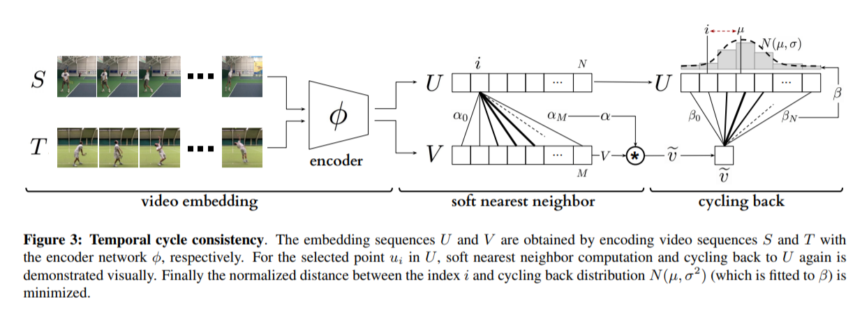 # Datasets All training is done in a self-supervised fashion. To evaluate their methods, they annotate the Pouring dataset, which they introduce and the Penn Action dataset. To annotate the datasets, they limit labels to specific events and phases between phases  # Model The network consists of two parts: an encoder network and an embedder network. ## Encoder They experiment with two encoders: * ResNet-50 pretrained on imagenet. They use conv_4 layer's output which is 14x14x1024 as the encoder scheme. * A Vgg-like model from scratch whose encoder output is 14x14x512. ## Embedder They then fuse the k following frame encodings along the time dimension, and feed it to an embedder network which uses 3D Convolutions and 3D pooling to reduce it to a 1x128 feature vector. They find that k=2 works pretty well. 
1 Comments
|
Show, Attend and Tell: Neural Image Caption Generation with Visual Attention
Xu, Kelvin and Ba, Jimmy and Kiros, Ryan and Cho, Kyunghyun and Courville, Aaron C. and Salakhutdinov, Ruslan and Zemel, Richard S. and Bengio, Yoshua
International Conference on Machine Learning - 2015 via Local Bibsonomy
Keywords: dblp
Xu, Kelvin and Ba, Jimmy and Kiros, Ryan and Cho, Kyunghyun and Courville, Aaron C. and Salakhutdinov, Ruslan and Zemel, Richard S. and Bengio, Yoshua
International Conference on Machine Learning - 2015 via Local Bibsonomy
Keywords: dblp
|
[link]
# Summary The authors present a way to generate captions describing the content of images using attention-based mechanisms. They present two ways of training the network, one via standard backpropagation techniques and another using stochastic processes. They also show how their model can selectively "focus" on the relevant parts of an image to generate appropriate captions, as shown in the classic example of the famous woman throwing a frisbee. Finally, they validate their model on Flicker8k, Flicker30k and MSCOCO. 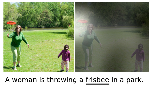 # Model At a very high level, the model takes as input an image I and returns a caption generated from a pre-defined vocabulary:  A high-level overview of the model is presented in Figure 1: 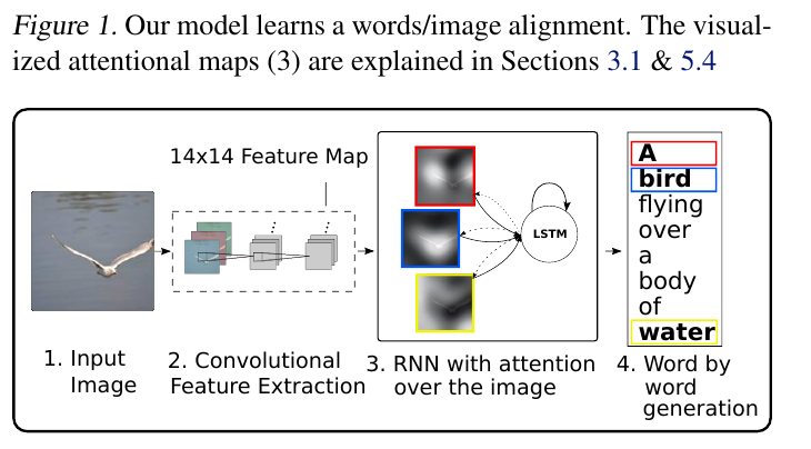 ## Visual extractor A CNN is used to extract features from the image. The authors experimented with VGG-19 pretrained on ImageNet and not finetuned. They use the features from the last convolutional layer as their representations. Starting with images of 224x224, the last CNN feature map has shape 14x14x512, which they flatten along width and height to obtain a vector representation of 196x512. These 512 vectors are used as inputs to the language model. ## Sentence generation An LSTM network is used to generate a sequence of words from a fixed vocabulary of size L. As input, a weighted sum based on attention values of the vectors of the flattened image features is used. The previous word is also fed as input to the LSTM. The hidden layer from the previous timestep as well as the layers from the CNN a_i are fed through an MLP + softmax layer and used to generate attention values for each flattened image feature vector that sum to one. 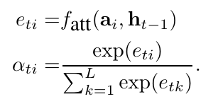  The authors propose two ways to compute phi, i.e. the attention, which they refer to as "soft attention" and "hard attention". These will be covered in a later section. The output of the LSTM, z, is then fed to a deep network to generate the next word. This is detailed in the following figure. 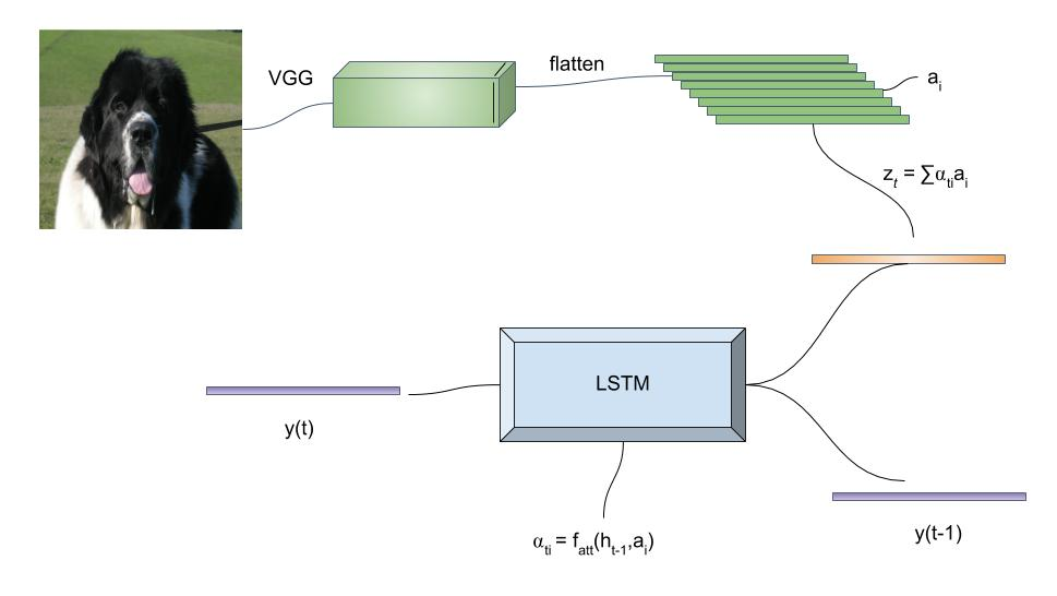 ## Attention The paper proposes two methods of attention, a "soft" attention and a "hard" attention. ### Soft attention Soft attention is the most intuitive one and is relatively straight forward. In order to compute the vector representing the image as input to the LSTM, **z**, the expectation of the context vector is computed by using a weighted average scheme: 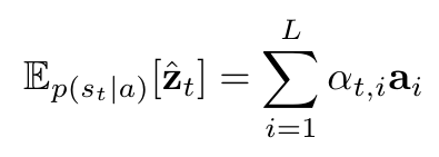 where alpha are the attention weights and a_i are the vectors of the feature representation. To ensure that all image features are used somewhat equally, a regularization term is added to the loss function:  This ensures that the image feature vectors over time sum to 1 as closely as possible and that no part of the image is ignored. ### Hard attention The authors propose an alternative method to calculate attention. Each attention parameter is treated as an intermediate latent variables that can be represented in one-hot encoding, i.e. on or off. To do so, they use a multinoulli distribution parametrized by alpha, the softmax output of f_att. They show how they can approximate the gradient using monte-carlo methods: 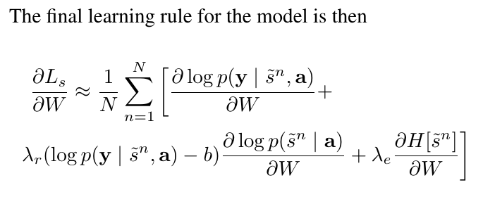 Refer to the paper for more mathemagical details. Finally, they use soft attention with probability 0.5 when using hard attention. ## Visualizing features One of the contributions of this work is showing what the network is "attending" to. To do so, the authors use the final layer of VGG-19, which consists of 14x14x512 features, upsample the resulting filters to the original image size of 224x224 and use a Gaussian blur to recreate the receptive field. ## Results The authors evaluate their methods on 3 caption datasets, i.e. Flicker8k, Flicker30k and MSCOCO. For all our experiments, they used a fixed vocabulary size of 10,000. They report both BLEU and METEOR scores on the task. As can be seen in the following figure, both the soft and hard attention mechanisms beat all state of the art methods at the time of publishing. Hard attention outperformed soft attention most of the time. 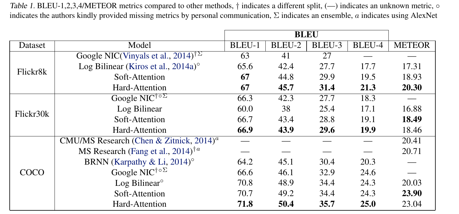 # Comments Cool paper which lead the way in terms of combining text and images and using attention mechanisms. They show an interesting way to visualize what the network is attending to, although it was not clear to me why they should expect the final layer of the CNN to be showing that in the first place since they did not finetune on the datasets they were training on. I would expect that to mean that their method would work best on datasets most "similar" to ImageNet. Their hard attention mechanism seems a lot more complicated than the soft attention mechanism and it isn't always clear that it is much better other than it offers a stronger regularization and a type of dropout.  |
Bottom-Up and Top-Down Attention for Image Captioning and Visual Question Answering
Peter Anderson and Xiaodong He and Chris Buehler and Damien Teney and Mark Johnson and Stephen Gould and Lei Zhang
Conference and Computer Vision and Pattern Recognition - 2018 via Local CrossRef
Keywords:
Peter Anderson and Xiaodong He and Chris Buehler and Damien Teney and Mark Johnson and Stephen Gould and Lei Zhang
Conference and Computer Vision and Pattern Recognition - 2018 via Local CrossRef
Keywords:
|
[link]
# Summary This paper presents state-of-the-art methods for both caption generation of images and visual question answering (VQA). The authors build on previous methods by adding what they call a "bottom-up" approach to previous "top-down" attention mechanisms. They show that using their approach they obtain SOTA on both Image captioning (MSCOCO) and the Visual Question and Answering (2017 VQA challenge). They propose a specific network configurations for each. Their biggest contribution is using Faster-R-CNN to retrieve the "important" parts of an image to focus on in both models. ## Top Down Up until this paper, the traditional approach was to use a "top-down" approach, in which the last feature map layer of a CNN is used to obtain a latent representation of the given input image. These features, along with the context of the caption being generated, were used to generate attention weights that were used to predict the next sequence in the context of caption generation. The network would learn to focus its attention on regions of the feature map that matters most. This is the approach used in previous SOTA methods like [Show, Attend and Tell: Neural Image Caption Generation with Visual Attention](https://arxiv.org/abs/1502.03044). ## Bottom-up The authors argue that the feature map of a CNN is too generic and can be thought of operating on a uniform, grid-like feature map. In other words, there is no particular reason to think that the feature map of generated by a CNN would give optimal regions to attend to. Also, carefully choosing the dimensions of the feature map can be very arbitrary. In order to fix this, the authors propose combining object detection methods in a *bottom-up* approach. To do so, the authors propose using Faster-R-CNN to identify regions of interest in an image. Given an input image, Faster-R-CNN will identify bounding boxes of the image that likely correspond to objects of a given category and simultaneously compute a feature vector of that bounding box. Figure 1 shows the difference between the Bottom-up and Top-Down approach. 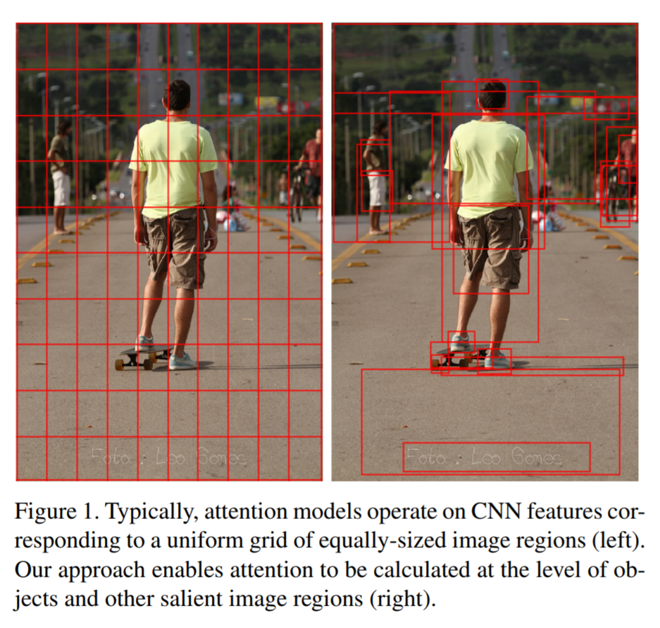 ## Combining the two In this paper, the authors suggest using the bottom-up approach to compute the salient regions of the image the network should focus on using Faster-R-CNN. FRCNN is carefully pretrained on both imagenet and the Visual Genome dataset. It is then frozen and only used to generate bounding boxes of regions with high confidence of being of interest. The top-down approach is then used on the features obtained from the bottom-up approach. In order to "enhance" the FRCNN performance, they initialize their FRCNN with a ResNet-101 pre-trained on imagenet. They train their FRCNN on the Visual Genome dataset, adding attributes to the loss function that are available from the Visual Genome dataset, attributes such as color (black, white, gold etc.), state (open, close, dark, bright, etc.). A sample of FRCNN outputs are shown in figure 2. It is important to stress that only the feature representations and not the actual outputs (i.e. not the labels) are used in their model. 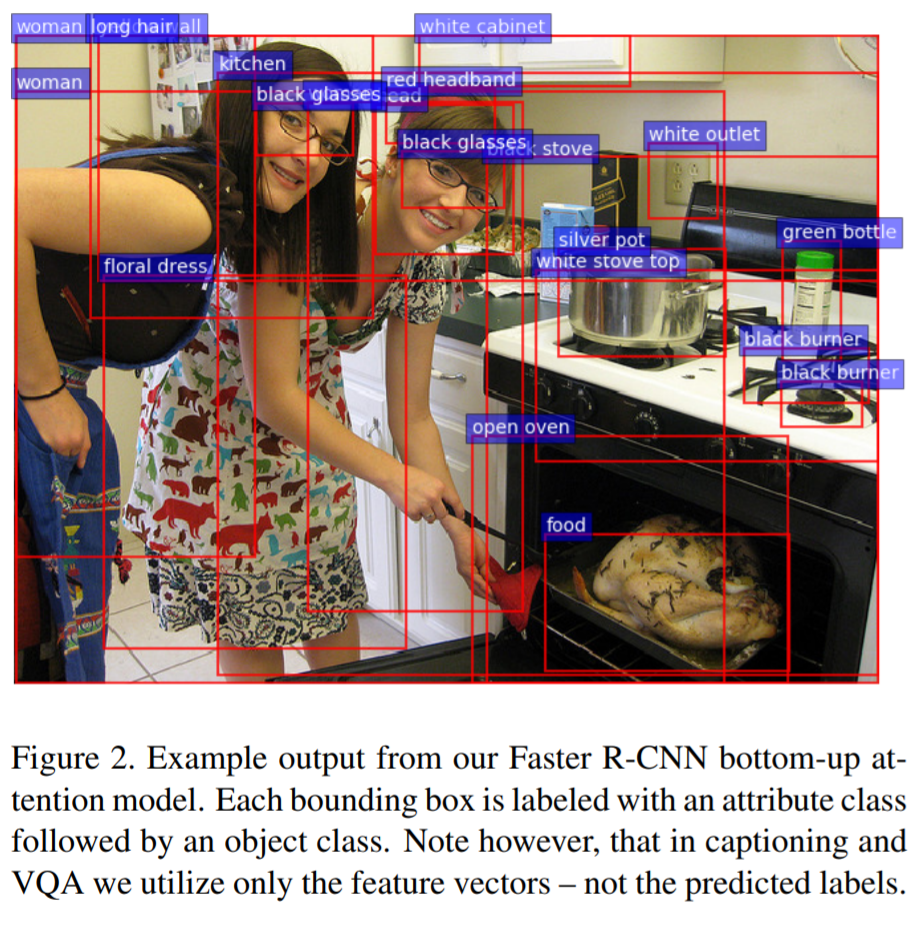 ## Caption Generation Figure 3 provides a high-level overview of the model being used for caption generation for images. The image is first passed through FRCNN which produces a set of image features *V*. In their specific implementation, *V* consists of *k* vectors of size 1x2048. Their model consists of two LSTM blocks, one for attention and the other for language generation. 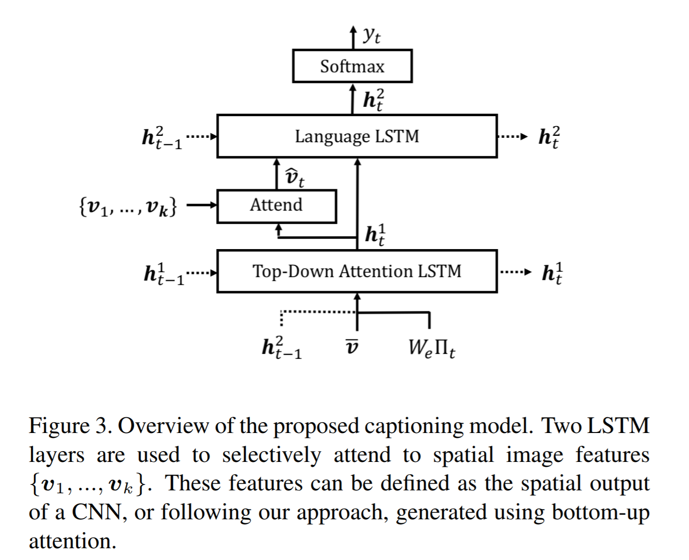 The first block of their model is a Top-Down Attention LSTM layer. It takes as input the mean-pooled features *V* , i.e. 1/k*sum(v_i), concatenated with the previous timestep's hidden representation of the language LSTM as well as the word embedding of the previously generated word. The word embedding is learned and not pretrained. The output of the first LSTM is used to compute the attention for each vector using an MLP and softmax: 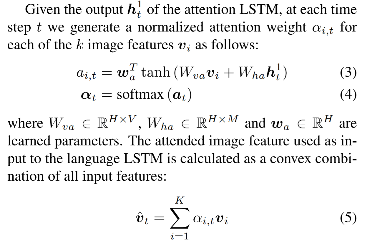 The attention weighted image feature is then used as an input to the language LSTM model, concatenated with the output from the top-down Attention LSTM and a softmax is used to predict the next word in the sequence. The loss function seeks to minimize the cross-entropy of the generated sentence. ## VQA Model The VQA task differs to the image generation in that a text-based question accompanies an input image and the network must produce an answer. The VQA model proposed is different to that of the caption generation model previously described, however they both use the same bottom-up approach to generate the feature vectors of the image based on the FRCNN architecture. A high-level overview of the architecture for the VQA model is presented in Figure 4.  Each word from the question is converted to a learned word embedding which is used as input to a GRU. The number of words for each question is limited to 14 for computational efficiency. The output from the GRU is concatenated with each of the *k* image features, and attention weights are computed for each *k*th feature using an MLP and softmax, similar to what is done in the attention for caption generation. The weighted sum of the feature vectors is then passed through an linear layer such that its shape is compatible with the gru output, and the Hadamard product (element-wise product) is computed over the GRU output and attention-weighted image feature representation. Finally, a tanh non-linear activation is used. This results in a "gated tanh", which have been shown empirically to outperform both ReLU and tanh. Finally, a softmax probability distribution is generated at the output which selects a candidate answer among all possible candidate answers. ## Results and experiments ### Resnet Baseline To demonstrate that their contribution of bottom-up mechanism actually improves on results, the authors use a ResNet trained on imagenet as a baseline for generating the image feature vectors (they resize the final CNN layers using bilinear interpolation when needed). They consistently obtain better results when using the bottom-up approach over the ResNet approach in both caption generation and VQA. ## MSCOCO The authors demonstrate that they outperform all results on all metrics on the MSCOCO test server.  They also show how using the bottom-up approach over ResNet consistently scores them higher on detecting instances of objects, attributes, relations, etc:  The authors, like their predecessors, insist on demonstrating their network's frisbee ability: 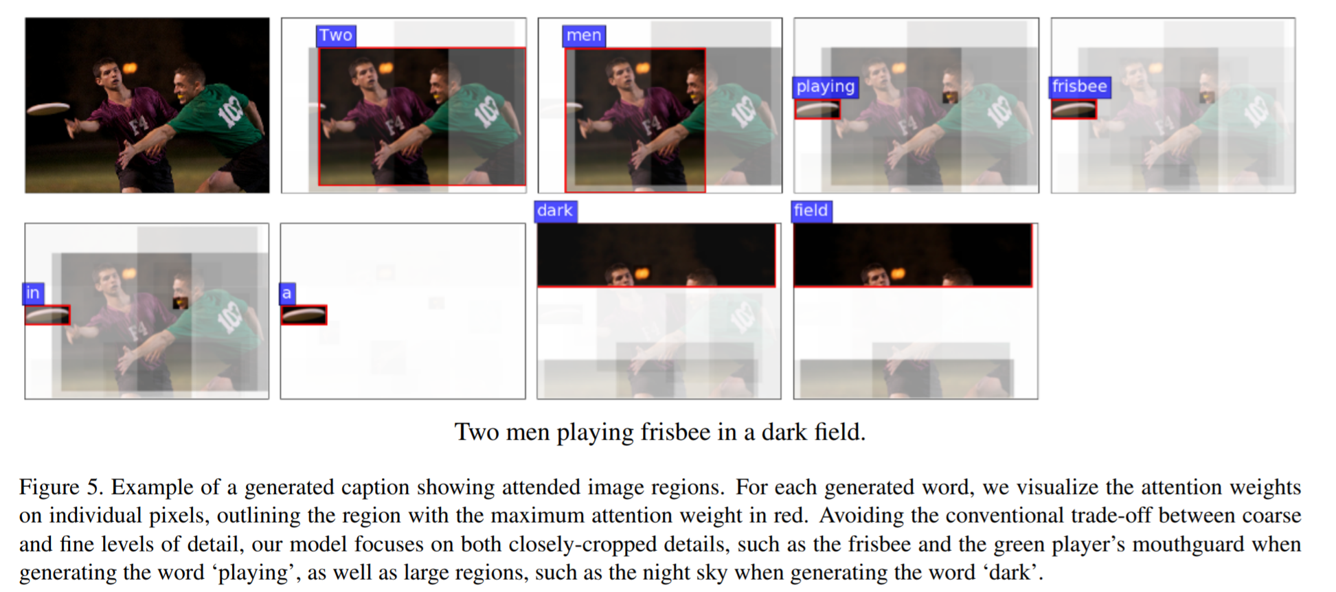 ## VQA Results They also demonstrate that the addition of bottom-up attention improves results over a ResNet baseline. 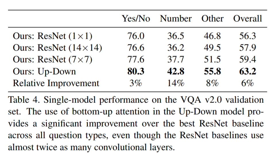 They also show that their model outperformed all other submissions on the VQA submission. They mention using an ensemble of 30 models for their submission. 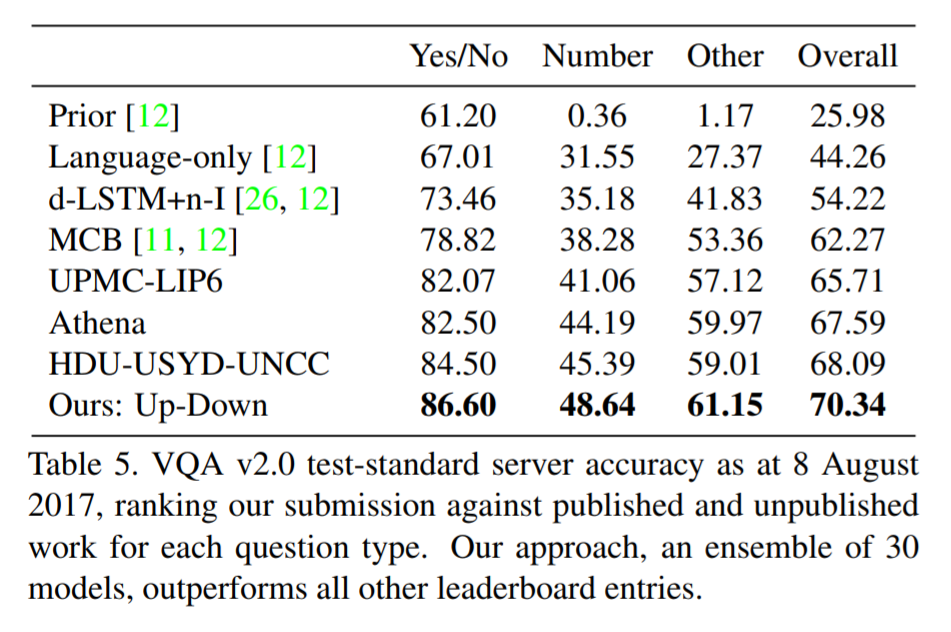 A sample image of what is attended in an image given a proper answer is shown in figure 6. 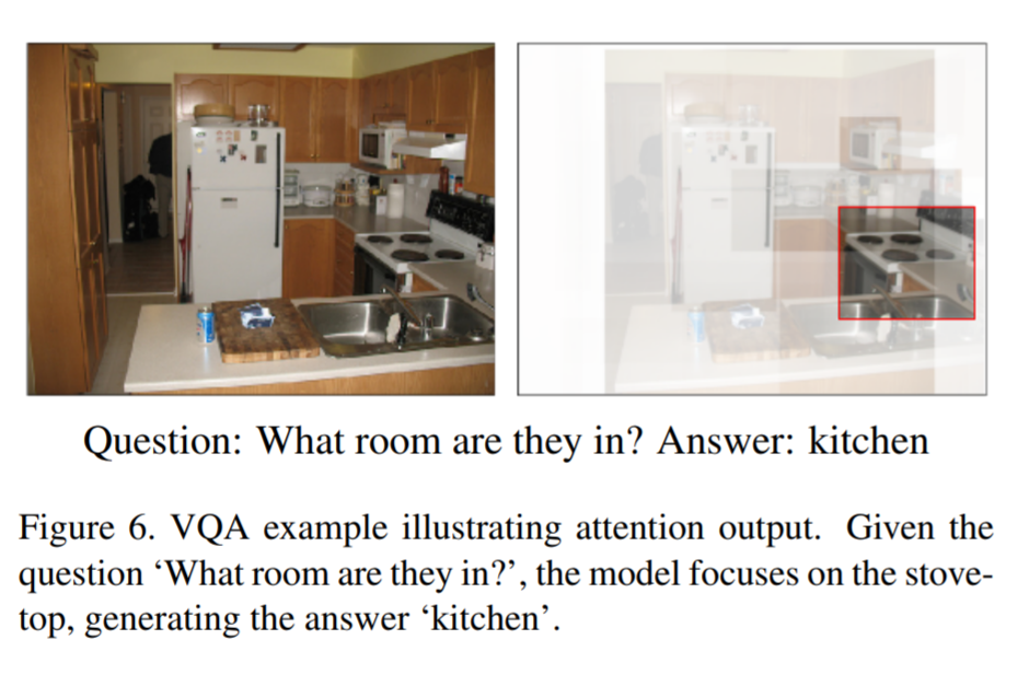 # Comments The authors introduce a new way to select portions of the image on which to focus attention. The idea is very original and came at a time when object detection was making significant progress (i.e. FRCNN). A few comments: * This method might not generalize well to other types of data. It requires pre-training on larger datasets (visual genome, imagenet, etc.) which consist of categories that overlap with both the MSCOCO and VQA datasets (i.e. cars, people, etc.). It would be interesting to see an end-to-end model that does not rely on pre-training on other similar datasets. * No insight is given to the computational complexity nor to the inference time or training time. I imagine that FRCNN is resource intensive, and having to do a forward pass of FRCNN for every pass of the network must be a computational bottleneck. Not to mention that they ensembled 30 of them!  |


