When machine learning models need to run on personal devices, that implies a very particular set of constraints: models need to be fairly small and low-latency when run on a limited-compute device, without much loss in accuracy. A number of human-designed architectures have been engineered to try to solve for these constraints (depthwise convolutions, inverted residual bottlenecks), but this paper's goal is to use Neural Architecture Search (NAS) to explicitly optimize the architecture against latency and accuracy, to hopefully find a good trade-off curve between the two. 

This paper isn't the first time NAS has been applied on the problem of mobile-optimized networks, but a few choices are specific to this paper. 

1. Instead of just optimizing against accuracy, or optimizing against accuracy with a sharp latency requirement, the authors here construct a weighted loss that includes both accuracy and latency, so that NAS can explore the space of different trade-off points, rather than only those below a sharp threshold.  
2. They design a search space where individual sections or "blocks" of the network can be configured separately, with the hope being that this flexibility helps NAS trade off complexity more strongly in the early parts of the network, where, at a higher spatial resolution, it implies greater computation cost and latency, without necessary dropping that complexity later in the network, where it might be lower-cost. Blocks here are specified by the type of convolution op, kernel size, squeeze-and-excitation ratio, use of a skip op, output filter size, and the number of times an identical layer of this construction will be repeated to constitute a block. 

Mechanically, models are specified as discrete strings of tokens (a block is made up of tokens indicating its choices along these design axes, and a model is made up of multiple blocks). These are represented in a RL framework, where a RNN model sequentially selects tokens as "actions" until it gets to a full model specification . This is repeated multiple times to get a batch of models, which here functions analogously to a RL episode. These models are then each trained for only five epochs (it's desirable to use a full-scale model for accurate latency measures, but impractical to run its full course of training). After that point, accuracy is calculated, and latency determined by running the model on an actual Pixel phone CPU. These two measures are weighted together to get a reward, which is used to train the RNN model-selection model using PPO. 

https://i.imgur.com/dccjaqx.png

Across a few benchmarks, the authors show that models found with MNasNet optimization are able to reach parts of the accuracy/latency trade-off curve that prior techniques had not.

Hosseini and Poovendran propose semantic adversarial examples by randomly manipulating hue and saturation of images. In particular, in an iterative algorithm, hue and saturation are randomly perturbed and projected back to their valid range. If this results in mis-classification the perturbed image is returned as the adversarial example and the algorithm is finished; if not, another iteration is run. The result is shown in Figure 1. As can be seen, the structure of the images is retained while hue and saturation changes, resulting in mis-classified images.

https://i.imgur.com/kFcmlE3.jpg
Figure 1: Examples of the computed semantic adversarial examples.

Also find this summary at [davidstutz.de](https://davidstutz.de/category/reading/).

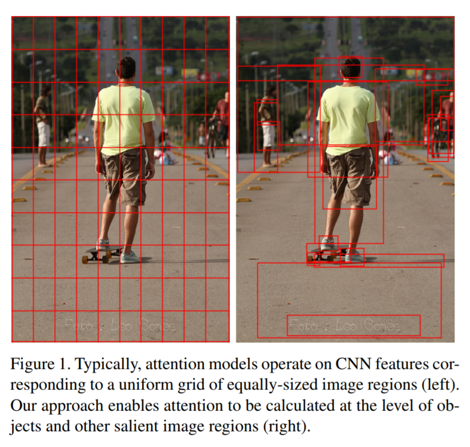
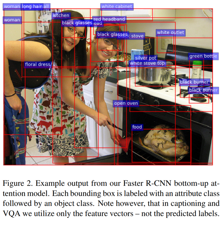
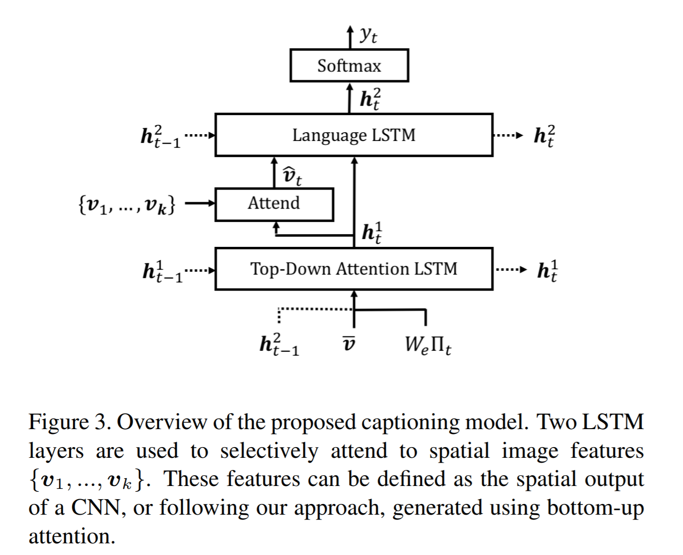
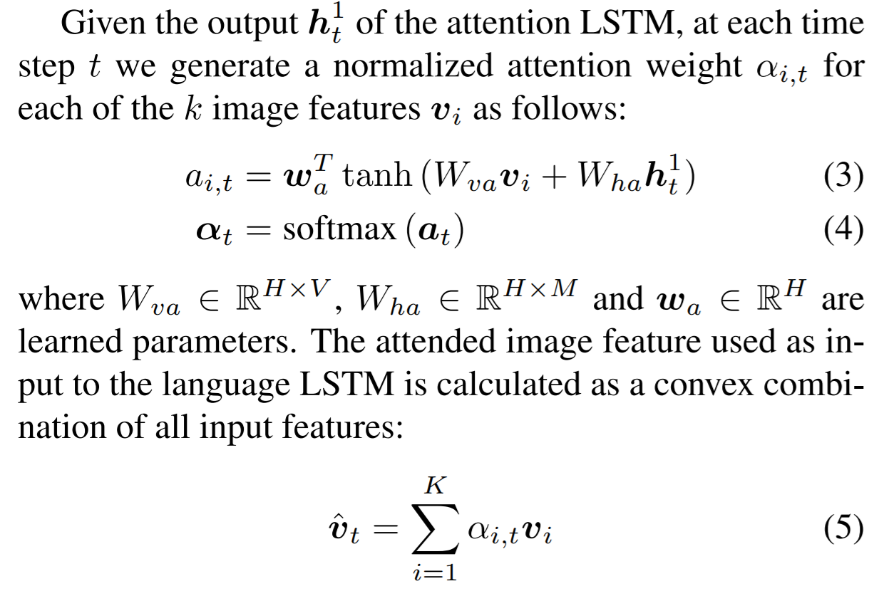
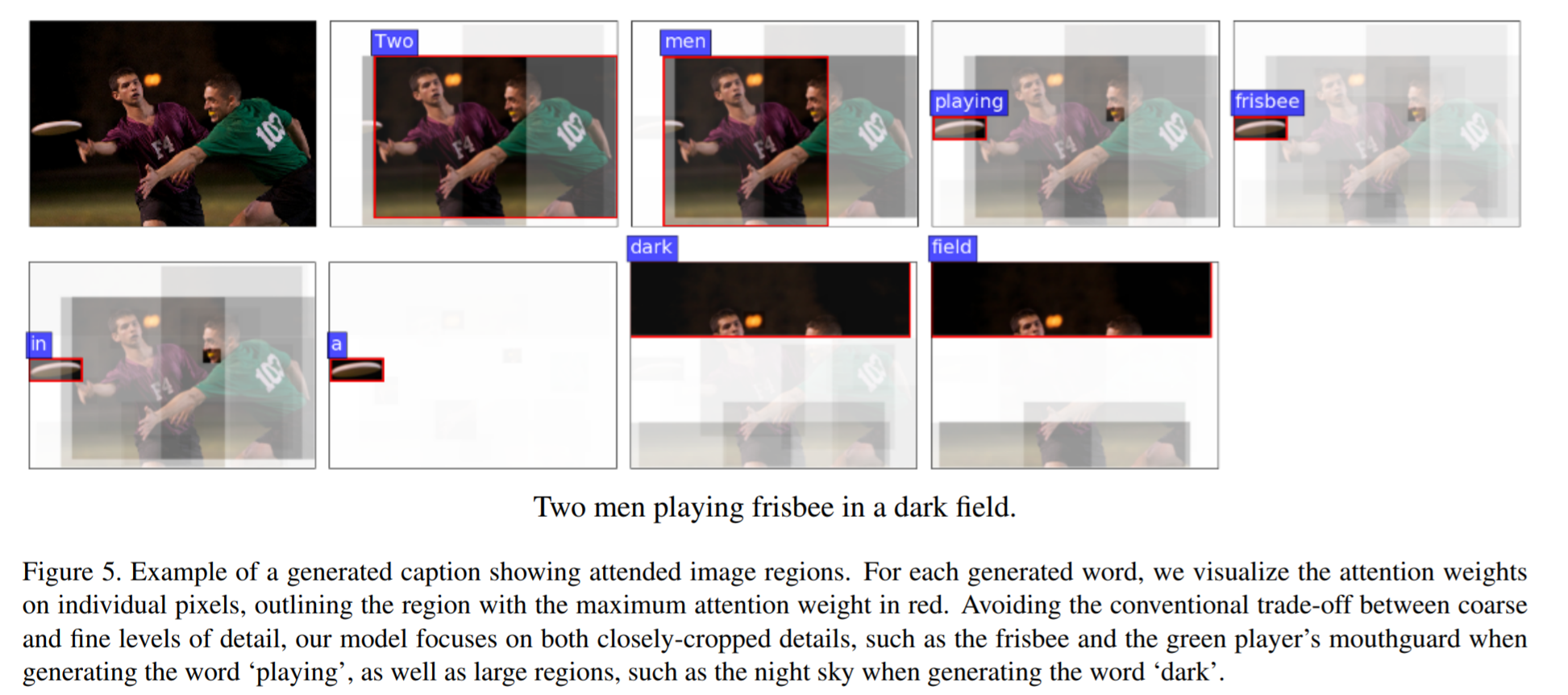
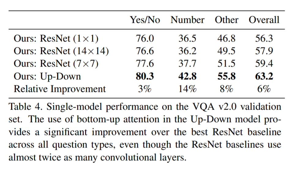
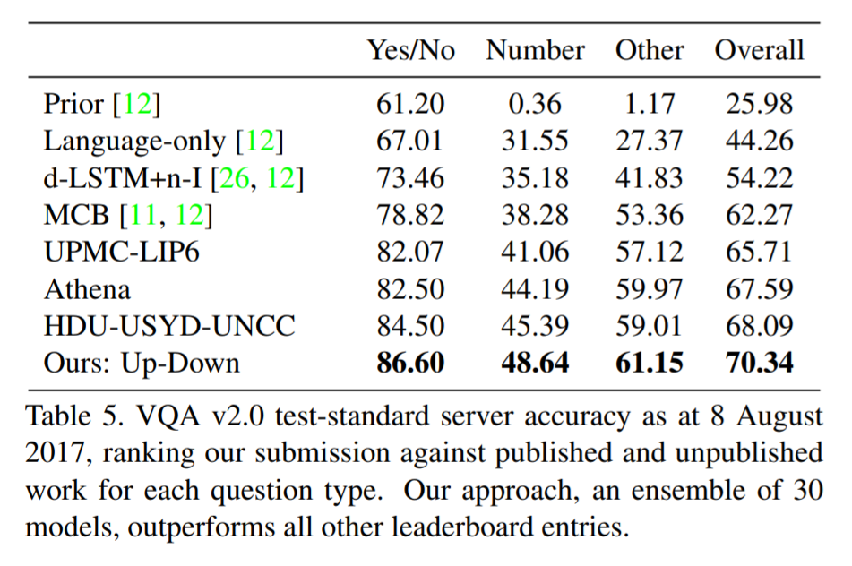
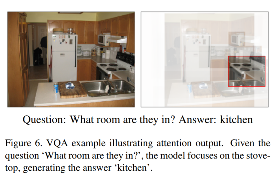
# Summary

This paper presents state-of-the-art methods for both caption generation of images and visual question answering (VQA). The authors build on previous methods by adding what they call a "bottom-up" approach to previous "top-down" attention mechanisms. They show that using their approach they obtain SOTA on both Image captioning (MSCOCO) and the Visual Question and Answering (2017 VQA challenge). They propose a specific network configurations for each. Their biggest contribution is using Faster-R-CNN to retrieve the "important" parts of an image to focus on in both models.

## Top Down

Up until this paper, the traditional approach was to use a "top-down" approach, in which the last feature map layer of a CNN is used to obtain a latent representation of the given input image. These features, along with the context of the caption being generated, were used to generate attention weights that were used to predict the next sequence in the context of caption generation. The network would learn to focus its attention on regions of the feature map that matters most. This is the approach used in previous SOTA methods like [Show, Attend and Tell: Neural Image Caption Generation with Visual Attention](https://arxiv.org/abs/1502.03044).

## Bottom-up

The authors argue that the feature map of a CNN is too generic and can be thought of operating on a uniform, grid-like feature map. In other words, there is no particular reason to think that the feature map of generated by a CNN would give optimal regions to attend to. Also, carefully choosing the dimensions of the feature map can be very arbitrary.

In order to fix this, the authors propose combining object detection methods in a *bottom-up* approach. To do so, the authors propose using Faster-R-CNN to identify regions of interest in an image. Given an input image, Faster-R-CNN will identify bounding boxes of the image that likely correspond to objects of a given category and simultaneously compute a feature vector of that bounding box. Figure 1 shows the difference between the Bottom-up and Top-Down approach.

![image](https://user-images.githubusercontent.com/18450628/61817263-2683cd00-ae1c-11e9-971a-d3b531dbbd98.png)

## Combining the two

In this paper, the authors suggest using the bottom-up approach to compute the salient regions of the image the network should focus on using Faster-R-CNN. FRCNN is carefully pretrained on both imagenet and the Visual Genome dataset. It is then frozen and only used to generate bounding boxes of regions with high confidence of being of interest. The top-down approach is then used on the features obtained from the bottom-up approach. In order to "enhance" the FRCNN performance, they initialize their FRCNN with a ResNet-101 pre-trained on imagenet. They train their FRCNN on the Visual Genome dataset, adding attributes to the loss function that are available from the Visual Genome dataset, attributes such as color (black, white, gold etc.),  state (open, close, dark, bright, etc.). A sample of FRCNN outputs are shown in figure 2. It is important to stress that only the feature representations and not the actual outputs (i.e. not the labels) are used in their model.

![image](https://user-images.githubusercontent.com/18450628/61817487-aca01380-ae1c-11e9-90fa-134033b95bb0.png)

## Caption Generation

Figure 3 provides a high-level overview of the model being used for caption generation for images. The image is first passed through FRCNN which produces a set of image features *V*. In their specific implementation, *V* consists of *k* vectors of size 1x2048. Their model consists of two LSTM blocks, one for attention and the other for language generation.

![image](https://user-images.githubusercontent.com/18450628/61818488-effb8180-ae1e-11e9-8ae4-14355115429a.png)

The first block of their model is a Top-Down Attention LSTM layer. It takes as input the mean-pooled features *V* , i.e. 1/k*sum(v_i), concatenated with the previous timestep's hidden representation of the language LSTM as well as the word embedding of the previously generated word. The word embedding is learned and not pretrained. 

The output of the first LSTM is used to compute the attention for each vector using an MLP and softmax:

![image](https://user-images.githubusercontent.com/18450628/61819982-21298100-ae22-11e9-80a9-99640896413d.png)

The attention weighted image feature is then used as an input to the language LSTM model, concatenated with the output from the top-down Attention LSTM and a softmax is used to predict the next word in the sequence. The loss function seeks to minimize the cross-entropy of the generated sentence. 

## VQA Model

The VQA task differs to the image generation in that a text-based question accompanies an input image and the network must produce an answer. The VQA model proposed is different to that of the caption generation model previously described, however they both use the same bottom-up approach to generate the feature vectors of the image based on the FRCNN architecture. A high-level overview of the architecture for the VQA model is presented in Figure 4.

![image](https://user-images.githubusercontent.com/18450628/61821988-8da67f00-ae26-11e9-8456-3c9e5ec60787.png)

Each word from the question is converted to a learned word embedding which is used as input to a GRU. The number of words for each question is limited to 14 for computational efficiency. The output from the GRU is concatenated with each of the *k* image features, and attention weights are computed for each *k*th feature using an MLP and softmax, similar to what is done in the attention for caption generation. The weighted sum of the feature vectors is then passed through an linear layer such that its shape is compatible with the gru output, and the Hadamard product (element-wise product) is computed over the GRU output and attention-weighted image feature representation. Finally, a tanh non-linear activation is used. This results in a "gated tanh", which have been shown empirically to outperform both ReLU and tanh. Finally, a softmax probability distribution is generated at the output which selects a candidate answer among all possible candidate answers.

## Results and experiments

### Resnet Baseline

To demonstrate that their contribution of bottom-up mechanism actually improves on results, the authors use a ResNet trained on imagenet as a baseline for generating the image feature vectors (they resize the final CNN layers using bilinear interpolation when needed). They consistently obtain better results when using the bottom-up approach over the ResNet approach in both caption generation and VQA.

## MSCOCO

The authors demonstrate that they outperform all results on all metrics on the MSCOCO test server.

![image](https://user-images.githubusercontent.com/18450628/61824157-4f5f8e80-ae2b-11e9-8d90-657db453e26e.png)

They also show how using the bottom-up approach over ResNet consistently scores them higher on detecting instances of objects, attributes, relations, etc:

![image](https://user-images.githubusercontent.com/18450628/61824238-7fa72d00-ae2b-11e9-81b3-b5a7f80153f3.png)

The authors, like their predecessors, insist on demonstrating their network's frisbee ability:

![image](https://user-images.githubusercontent.com/18450628/61824344-bed57e00-ae2b-11e9-87cd-597568587e1d.png)

## VQA Results

They also demonstrate that the addition of bottom-up attention improves results over a ResNet baseline. 

![image](https://user-images.githubusercontent.com/18450628/61824500-28ee2300-ae2c-11e9-9016-2120a91917e4.png)

They also show that their model outperformed all other submissions on the VQA submission. They mention using an ensemble of 30 models for their submission. 

![image](https://user-images.githubusercontent.com/18450628/61824634-83877f00-ae2c-11e9-8d84-9589e0ea2be2.png)


A sample image of what is attended in an image given a proper answer is shown in figure 6.

![image](https://user-images.githubusercontent.com/18450628/61824608-736f9f80-ae2c-11e9-9d4e-8cb6bd0a1a92.png)


# Comments

The authors introduce a new way to select portions of the image on which to focus attention. The idea is very original and came at a time when object detection was making significant progress (i.e. FRCNN).

A few comments:

* This method might not generalize well to other types of data. It requires pre-training on larger datasets (visual genome, imagenet, etc.) which consist of categories that overlap with both the MSCOCO and VQA datasets (i.e. cars, people, etc.). It would be interesting to see an end-to-end model that does not rely on pre-training on other similar datasets.

* No insight is given to the computational complexity nor to the inference time or training time. I imagine that FRCNN is resource intensive, and having to do a forward pass of FRCNN for every pass of the network must be a computational bottleneck. Not to mention that they ensembled 30 of them!

Sharif et al. study the effectiveness of $L_p$ norms for creating adversarial perturbations. In this context, their main discussion revolves around whether $L_p$ norms are sufficient and/or necessary for perceptual similarity. Their main conclusion is that $L_p$ norms are neither necessary nor sufficient to ensure perceptual similarity. For example, an adversarial example might be within a specific $L_p$ bal, but humans might still identify it as not similar enough to the originally attacked sample; on the other hand, there are also some imperceptible perturbations that usually extend beyond a reasonable $L_p$ ball. Such transformatons might for example include small rotations or translation. These findings are interesting because it indicates that our current model, or approximation, or perceptual similarity is not meaningful in all cases.

Also find this summary at [davidstutz.de](https://davidstutz.de/category/reading/).

Dong et al. introduce momentum into iterative white-box adversarial examples and also show that attacking ensembles of models improves transferability. Specifically, their contribution is twofold. First, some iterative white-box attacks are extended to include a momentum term. As in optimization or learning, the main motivation is to avoid local maxima and have faster convergence. In experiments, they show that momentum is able to increase the success rates of attacks.

Second, to improve the transferability of adversarial examples in black-box scenarios, Dong et al. propose to compute adversarial examples on ensembles of models. In particular, the logits of multiple models are summed (optionally using weights) and attacks are crafter to fool multiple models at once. In experiments, crafting adversarial examples on an ensemble of diverse networks allows higher success rate sin black-box scenarios.

Also find this summary at [davidstutz.de](https://davidstutz.de/category/reading/).

Akhtar et al. Propose a rectification and detection scheme as defense against universal adversarial perturbations. Their overall approach is illustrated in Figure 1 an briefly summarized as follows. Given a classifier with fixed weights, a rectification network (the so-called perturbation rectifying network – PRN) is trained in order to “undo” the perturbations. This network can be trained on a set of clean and perturbed images using the classifier’s loss. Second, based on the discrete cosine transform (DCT) of the difference between original and rectified image (both for clean and perturbed images), a SVM is trained to detect adversarially perturbed images. At test time, only images that have been identified as being perturbed are rectified. In experiments, the authors show that this setup is able to defend against adversarial attacks and does not influence the classifier’s accuracy significantly.

https://i.imgur.com/KzY7Wwr.png
Figure 1: The proposed perturbation rectifying network (PRN) asnd the correcponding perturbation detector.

Overall, the proposed approach is comparable to other work that tries to either detect adversarial perturbations, or to remove them from the test image. One advantage is that the classifier itself does not need to be re-trained. However, as the rectification network is itself a (convolutional) neural netowrk, and the detector is a SVM, both are also potential targets of attacks – althoguh attacking the whole system might be more challenging (especially crafting universal perturbations).

Also find this summary at [davidstutz.de](https://davidstutz.de/category/reading/).

## Task
They introduce a dense version of the human pose estimation task: predict body surface coordinates for each pixel in an RGB image.

Body surface is representated on two levels:
- Body part label (24 parts)
    - Head, torso, hands, feet, etc.
    - Each leg split in 4 parts: upper/lower front/back. Same for arms.
- 2 coordinates (u,v) within body part
    - head, hands, feet: based on SMPL model
    - others: determined by Multidimensional Scaling on geodesic distances

## Data
* They annotate COCO for this task
    - annotation tool: draw mask, then click on a 3D rendering for each of up to 14 points sampled from the mask
    - annotator accuracy on synthetic renderings (average geodesic distance)
       - small parts (e.g. feet): ~2 cm
       - large parts (e.g. torso): ~7 cm

## Method

Fully-convolutional baseline
  - ResNet-50/101
  - 25-way body part classification head (cross-entropy loss)
  - Regression head with 24*2 outputs per pixel (Huber loss)

Region-based approach
  - Like Mask-RCNN
  - New branch with same architecture as the keypoint branch
  - ResNet-50-FPN (Feature Pyramid Net) backbone

Enhancements tested:

- Multi-task learning
  - Train keypoint/mask and dense pose task at once
  - Interaction implicit by sharing backbone net

- Multi-task *cross-cascading*
  - Explicit interaction of tasks
  - Introduce second stage that depends on the first-stage-output of all tasks

- Ground truth interpolation (distillation)
  - Train a "teacher" FCN with the pointwise annotations
  - Use its dense predictions as ground truth to train final net
  - (To make the teacher as accurate as possible, they use ground-truth mask to remove background)

## Results

**Single-person results (train and test on single-person crops)**

Pointwise eval measure:
   - Compute geodesic distance between prediction and ground truth at each annotated point
   - For various error thresholds, plot percentage of points with lower error than the threshold
   - Compute Area Under this Curve

Training (non-regional) FCN on new dataset vs. synthetic data improves AUC10 from 0.20 to 0.38

This paper's FCN method vs. model-fitting baseline
- Baseline: Estimate body keypoint locations in 2D (usual "pose estimation" task) + fit 3D model
- AUC10 improves from 0.23 to 0.43
- Speed: 4-25 fps for FCN vs. model-fitting taking 1-3 minutes per frame (!).

**Multi-person results**

- Region-based method outperforms FCN baseline: 0.25 -> 0.32
    - FCN cannot deal well with varying person scales (despite multi-scale testing)
- Training on points vs interpolated ground-truth (distillation) 0.32 -> 0.38
- AUC10 with cross-task cascade: 0.39

Also: Per-instance eval ("Geodesic Point Similarity" - GPS)
   - Compute a Gaussian function on the geodesic distances
   - Average it within each person instance (=> GPS)
   - Compute precision and recall of persons for various thresholds of GPS
   - Compute average precision and recall over thresholds

Comparison of multi-task approaches:
1. Just dense pose branch (single-task) (AP 51)
2. Adding keypoint (AP 53) OR mask branch (multi-task without cross-cascade) (AP 52)
3. Refinement stage without cross-links (AP 52)
4. Multi-task cross-cascade (keypoints: AP 56, masks: AP 53)