Synthesizing the preferred inputs for neurons in neural networks via deep generator networks
Nguyen, Anh and Dosovitskiy, Alexey and Yosinski, Jason and Brox, Thomas and Clune, Jeff
Neural Information Processing Systems Conference - 2016 via Local Bibsonomy
Keywords: dblp
Nguyen, Anh and Dosovitskiy, Alexey and Yosinski, Jason and Brox, Thomas and Clune, Jeff
Neural Information Processing Systems Conference - 2016 via Local Bibsonomy
Keywords: dblp
|
[link]
This paper performs activation maximization (AM) using Deep Generator Network (DGN), which served as a learned natural iamge prior, to synthesize realistic images as inputs and feed it into the DNN we want to understand. By visualizing synthesized images that highly activate particular neurons in the DNN, we can interpret what each of neurons in the DNN learned to detect. ### Key Points - DGN (natural image prior) generates more coherent images when optimizing fully-connected layer codes instead of low-level codes. However, previous studies showed that low-level features results in better reconstructions beacuse it contains more image details. The difference is that here DGN-AM is trying to synthesize an entire layer code from scratch. Features in low-level only has a small, local receptive field so that the optimization process has to independently tune image without knowing the global structure. Also, the code space at a convolutional layer is much more high-dimensional, making it harder to optimize. - The learned prior trained on ImageNet can also generalize to Places. - It doesn't generalize well if architecture of the encoder trained with DGN is different with the DNN we wish to inspect. - The learned prior also generalizes to visualize hidden neurons, producing more realistic textures/colors. - When visualizing hidden neurons, DGN-AM trained on ImageNet also generalize to Places and produce similar results as [1]. - The synthesized images are showed to teach us what neurons in DNN we wish to inspect prefer instead of what prior prefer. ### Model  ### Thought Solid paper with diverse visualizations and thorough analysis. ### Reference [1] Object Detectors Emerge In Deep Scene CNNs, B.Zhou et. al. 
Your comment:
|
|
[link]
* They suggest a new method to generate images which maximize the activation of a specific neuron in a (trained) target network (abbreviated with "**DNN**").
* E.g. if your DNN contains a neuron that is active whenever there is a car in an image, the method should generate images containing cars.
* Such methods can be used to investigate what exactly a network has learned.
* There are plenty of methods like this one. They usually differ from each other by using different *natural image priors*.
* A natural image prior is a restriction on the generated images.
* Such a prior pushes the generated images towards realistic looking ones.
* Without such a prior it is easy to generate images that lead to high activations of specific neurons, but don't look realistic at all (e.g. they might look psychodelic or like white noise).
* That's because the space of possible images is extremely high-dimensional and can therefore hardly be covered reliably by a single network. Note also that training datasets usually only show a very limited subset of all possible images.
* Their work introduces a new natural image prior.
### How
* Usually, if one wants to generate images that lead to high activations, the basic/naive method is to:
1. Start with a noise image,
2. Feed that image through DNN,
3. Compute an error that is high if the activation of the specified neuron is low (analogous for high activation),
4. Backpropagate the error through DNN,
5. Change the noise image according to the gradient,
6. Repeat.
* So, the noise image is basically treated like weights in the network.
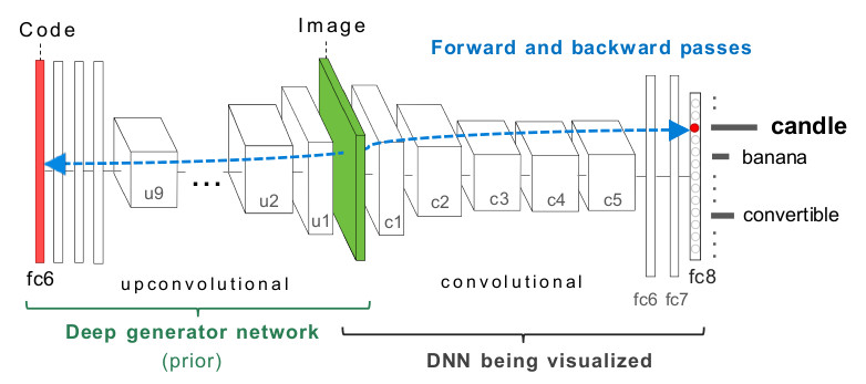
* Their alternative method is based on a Generator network **G**.
* That G is trained according to the method described in [Generating Images with Perceptual Similarity Metrics based on Deep Networks].
* Very rough outline of that method:
* First, a pretrained network **E** is given (they picked CaffeNet, which is a variation of AlexNet).
* G then has to learn to inverse E, i.e. G receives per image the features extracted by a specific layer in E (e.g. the last fully connected layer before the output) and has to generate (recreate) the image from these features.
* Their modified steps are:
1. *(New step)* Start with a noise vector,
2. *(New step)* Feed that vector through G resulting in an image,
3. *(Same)* Feed that image through DNN,
4. *(Same)* Compute an error that is low if the activation of the specified neuron is high (analogous for low activations),
5. *(Same)* Backpropagate the error through DNN,
6. *(Modified)* Change the noise *vector* according to the gradient,
7. *(Same)* Repeat.
* Visualization of their architecture:
* 
* Additionally they do:
* Apply an L2 norm to the noise vector, which adds pressure to each component to take low values. They say that this improved the results.
* Clip each component of the noise vector to a range `[0, a]`, which improved the results significantly.
* The range starts at `0`, because the network (E) inverted by their Generator (G) is based on ReLUs.
* `a` is derived from test images fed through E and set to 3 standard diviations of the mean activation of that component (recall that the "noise" vector mirrors a specific layer in E).
* They argue that this clipping is similar to a prior on the noise vector components. That prior reflects likely values of the layer in E that is used for the noise vector.
### Results
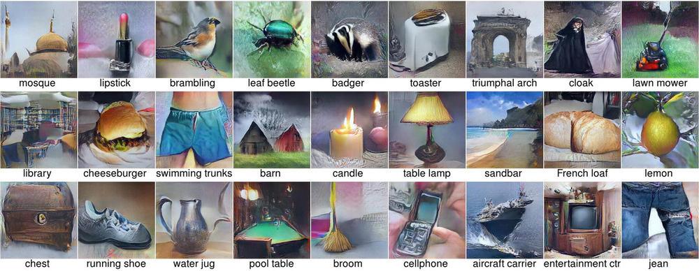
* Examples of generated images:
* 
* Early vs. late layers
* For G they have to pick a specific layer from E that G has to invert. They found that using "later" layers (e.g. the fully connected layers at the end) produced images with more reasonable overall structure than using "early" layers (e.g. first convolutional layers). Early layers led to repeating structures.
* Datasets and architectures
* Both G and DNN have to be trained on datasets.
* They found that these networks can actually be trained on different datasets, the results will still look good.
* However, they found that the architectures of DNN and E should be similar to create the best looking images (though this might also be down to depth of the tested networks).
* Verification that the prior can generate any image
* They tested whether the generated images really show what the DNN-neurons prefer and not what the Generator/prior prefers.
* To do that, they retrained DNNs on images that were both directly from the dataset as well as images that were somehow modified.
* Those modifications were:
* Treated RGB images as if they were BGR (creating images with weird colors).
* Copy-pasted areas in the images around (creating mosaics).
* Blurred the images (with gaussian blur).
* The DNNs were then trained to classify the "normal" images into 1000 classes and the modified images into 1000 other classes (2000 total).
* So at the end there were (in the same DNN) neurons reacting strongly to specific classes of unmodified images and other neurons that reacted strongly to specific classes of modified images.
* When generating images to maximize activations of specific neurons, the Generator was able to create both modified and unmodified images. Though it seemed to have some trouble with blurring.
* That shows that the generated images probably indeed show what the DNN has learned and not just what G has learned.
* Uncanonical images
* The method can sometimes generate uncanonical images (e.g. instead of a full dog just blobs of texture).
* They found that this seems to be mostly the case when the dataset images have uncanonical pose, i.e. are very diverse/multi-modal.
 |
You must log in before you can submit this summary! Your draft will not be saved!
Preview:


