[code](https://github.com/openai/improved-gan),
[demo](http://infinite-chamber-35121.herokuapp.com/cifar-minibatch/1/?),
[related](http://www.inference.vc/understanding-minibatch-discrimination-in-gans/)

### Feature matching
problem: overtraining on the current discriminator

solution:
$||E_{x \sim p_{\text{data}}}f(x) - E_{z \sim p_{z}(z)}f(G(z))||_{2}^{2}$

were f(x) activations intermediate layer in discriminator
### Minibatch discrimination
problem: generator to collapse to a single point

solution: for each sample i, concatenate to $f(x_i)$ features $b$ measuring its distance to other samples j (i and j are both real or generated samples in same batch):
$\sum_j \exp(-||M_{i, b} - M_{j, b}||_{L_1})$

this generates visually appealing samples very quickly
### Historical averaging
problem: SGD fails by going into extended orbits

solution: parameters revert to the mean
$|| \theta - \frac{1}{t} \sum_{i=1}^t \theta[i] ||^2$

### One-sided label smoothing
problem: discriminator vulnerability to adversarial examples

solution: discriminator target for positive samples is 0.9 instead of 1

### Virtual batch normalization
problem: using BN cause output of examples in batch to be dependent

solution: use reference batch chosen once at start of training and each sample is normalized using itself and the reference. It's
expensive so used only on generation

### Assessment of image quality
problem: MTurk not reliable

solution: use inception model p(y|x) to compute 
$\exp(\mathbb{E}_x \text{KL}(p(y | x) || p(y)))$
on 50K generated images x

### Semi-supervised learning
use the discriminator to also classify on K labels when known and
use all real samples (labels and unlabeled) in the discrimination task
$D(x) = \frac{Z(x)}{Z(x) + 1}, \text{ where } Z(x) = \sum_{k=1}^{K} \exp[l_k(x)]$.
In this case use feature matching but not minibatch discrimination.
It also improves the quality of generated images.

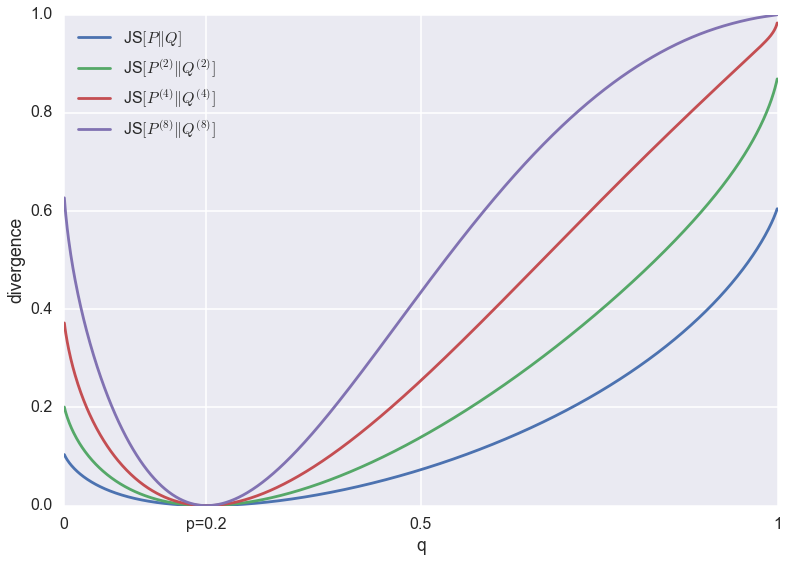
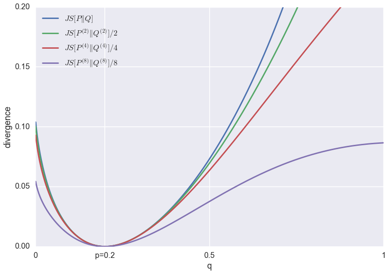
Summary of this post

 - How does this minibatch discrimination heuristic work and how does it change the behaviour of the GAN algorithm? Does it change the underlying objective function that is being minimized?
 - the answer is: for the original GAN algorithm that minimises Jensen-Shannon divergence it does change the behaviour in a non-trivial way. One side-effect is assigning a higher relative penalty for low-entropy generators.
 - when using the blended update rule from here, the algorithm minimises the reverse KL-divergence. In this case, using minibatch discrimination leaves the underlying objective unchanged: the algorithm can still be shown to miminise KL divergence.
 - even if the underlying objectives remain the same, using minibatch discrimination may be a very good idea practically. It may stabilise the algorithm by, for example, providing a lower variance estimator to log-probability-ratios.

[Here is the ipython/jupyter notebook](https://gist.github.com/fhuszar/a91c7d0672036335c1783d02c3a3dfe5) I used to draw the plots and test some of the things in this post in practice.

### What is minibatch discrimination?

In the vanilla Generative Adversarial Networks (GAN) algorithm, a discriminator is trained to tell apart generated synthetic examples from real data. One way GAN training can fail is to massively undershoot the entropy of the data-generating distribution, and concentrate all it's parameters on generating just a single or few examples.

To remedy this, the authors play with the idea of discriminating between whole minibatches of samples, rather than between individual samples. If the generator has low entropy, much lower than real data, it may be easier to detect this with a discriminator that sees multiple samples.

Here, I'm going to look at this technique in general: modifying an unsupervised learning algorithm by replacing individual samples with i.i.d. minibatches of samples. Note, that this is not exactly what the authors end up doing in the paper referenced above, but it's an interesting trick to think about.

#### How does the minibatch heuristic effect divergences?

The reason I'm so keen on studying GANs is the connection to principled information theoretic divergence criteria. Under some assumptions, it can be shown that GANs minimise the Jensen-Shannon (JS) divergence, or with a slight modification the reverse-KL divergence. In fact, a recent paper showed that you can use GAN-like algorithms to minimise any $f$-divergence.

So my immediate question looking at the minibatch discrimination idea was: how does this heuristic change the divergences that GANs minimise.

#### KL divergence

Let's assume we have any algorithm (GAN or anything else) that minimises KL divergence $\operatorname{KL}[P\|Q]$ between two distributions $P$ and $Q$. Let's now modify this algorithm so that instead of looking at distributions $P$ and $Q$ of a single sample $x$, it looks at distributions $P^{(N)}$ and $Q^{(N)}$ of whole a minibatch $(x_1,\ldots,x_N)$. I use $P^{(N)}$ to denote the following distribution:

$$ P^{(N)}(x_1,\ldots,x_N) = \prod_{n=1}^N P(x_n) 
$$

The resulting algorithm will therefore minimise the following divergence:

$$ d[P\|Q] = \operatorname{KL}[P^{(N)}\|Q^{(N)}] 
$$

It is relatively easy to show why this divergence $d$ behaves exactly like the KL divergence between $P$ and $Q$. Here's the maths for minibatch size of $N=2$:

\begin{align} d[P\|Q] &= \operatorname{KL}[P^{(2)}\|Q^{(2)}] \\ 
&= \mathbb{E}_{x_1\sim P,x_2\sim P}\log\frac{P(x_1)P(x_2)}{Q(x_1)Q(x_2)} \\ &= \mathbb{E}_{x_1\sim P,x_2\sim P}\log\frac{P(x_1)}{Q(x_1)} + \mathbb{E}_{x_1\sim P,x_2\sim P}\log\frac{P(x_2)}{Q(x_2)} \\ &= \mathbb{E}_{x_1\sim P}\log\frac{P(x_1)}{Q(x_1)} + \mathbb{E}_{x_2\sim P}\log\frac{P(x_2)}{Q(x_2)} \\ &= 2\operatorname{KL}[P\|Q] \end{align}

In full generality we can say that:

$$ \operatorname{KL}[P^{(N)}\|Q^{(N)}] = N \operatorname{KL}[P\|Q] $$

So changing the KL-divergence to minibatch KL-divergence does not change the objective of the training algorithm at all. Thus, if one uses minibatch discrimination with the blended training objective, one can rest assured that the algorithm still performs approximate gradient descent on the KL divergence. It may still work differently in practice, for example by reducing the variance of the estimators involved.

This property of the KL divergence is not surprising if one considers its compression/information theoretic definition: the extra bits needed to compress data drawn from $P$, using model $Q$. Compressing a minibatch of i.i.d. samples corresponds to compressing the samples independently. Their codelengths would add up linearly, hence KL-divergences add up linearly, too.

#### JS divergence

The same thing does not hold for the JS-divergence. Generally speaking, minibatch JS divergence behaves differently from ordinary JS-divergence. Instead of equality, for JS divergences the following inequality holds:

$$ JS[P^{(N)}\|Q^{(N)}] \leq N \cdot JS[P\|Q] 
$$

In fact for fixed $P$ and $Q$, $JS[P^{(N)}\|Q^{(N)}]/N$ is monotonically non-increasing. This can be seen intuitively by considering the definition of JS divergence as the mutual information between the samples and the binary indicator $y$ of whether the samples were drawn from $Q$ or $P$. Using this we have that:

\begin{align} \operatorname{JS}[P^{(2)}\|Q^{(2)}] &= \mathbb{I}[y ; x_1, x_2] \\ &= \mathbb{I}[y ; x_1] + \mathbb{I}[y ; x_2 \vert x_1] \\ &\leq \mathbb{I}[y ; x_1] + \mathbb{I}[y ; x_2] \\ &= 2 \operatorname{JS}[P\|Q] \end{align}

Below I plotted the minibatch-JS-divergence $JS[P^{(N)}\|Q^{(N)}]$ for various minibatch-sizes $N=1,2,3,8$, between univariate Bernoulli distributions with parameters $p$ and $q$. For the plots below, $p$ is kept fixed at $p=0.2$, and the parameter $q$ is varied between $0$ and $1$.

![](http://www.inference.vc/content/images/2016/06/fr9ra2qB2t9stl8sVnqIAAH1GqAAAhM3YsWOVkpKiTz75RD6fL9D-0UcfhbEqAEBfRYe7AABA5DIMQ-vXr9eLL76op556So8--qjOnDmjsrIyGYYR7vIAAL3ESAUAIKxmzpyp9957T52dndqyZYuOHTum4uJi7v4EAIMIIxUAgLCbPn26pk-fHtj2er1hrAYA0FeMVAAAAAAICaECAAAAQEgIFQCAm5JhGFysDQCDhOHnSjgAAAAAIWCkA.png)

You can see that all divergences have a unique global minimum around $p=q=0.2$. However, their behaviour at the tails changes as the minibatch-size increases. This change in behaviour is due to saturation: JS divergence is upper bounded by $1$, which corresponds to 1 bit of information. If I continued increasing the minibatch-size (which would blow up the memory footprint of my super-naive script), eventually the divergence would reach $1$ almost everywhere except for a dip down to $0$ around $p=q=0.2$.

Below are the same divergences normalised to be roughly the same scale.

![](http://www.inference.vc/content/images/2016/06/Rle8idcTS3gAAAABJRU5ErkJggg--.png)

The problem of GANs that minibatch discrimination was meant to fix is that it favours low-entropy solutions. In this plot, this would correspond to the $q<0.1$ regime. You can argue that as the batch-size increases, the relative penalty for low-entropy approximations $q<0.1$ do indeed decrease when compared to completely wrong solutions $q>0.5$. However, the effect is pretty subtle.

Bonus track: adversarial preference loss

In this context, I also revisited the adversarial preference loss. Here, the discriminator receives two inputs $x_1$ and $x_2$ (one synthetic, one real) and it has to decide which one was real.

This algorithm, too, can be related to the minibatch discrimination approach, as it minimises the following divergence:

$$ d(P,Q) = d(P\times Q\|Q\times P), 
$$

where $P\times Q(x_1,x_2) = P(x_1)Q(x_2)$. Again, if $d$ is the $KL$ divergence, the training objective boils down to the same thing as the original GAN. However, if $d$ is the JS divergence, we will end up minimising something weird, $\operatorname{JS}[Q\times P\| P\times Q]$

The Authors provide a bag of tricks for training GAN's in the image domain. Using these, they achieve very strong semi-supervised results on SHVN, MNIST, and CIFAR.

The authors then train the improved model on several images datasets, evaluate it on different tasks: semi-supervised learning, and generative capabilities, and achieve state-of-the-art results.

This paper investigates several techniques to stabilize GAN training and encourage convergence. Although lack of theoretical justification, the proposed heuristic techniques give better-looking samples. In addition to human judgement, the paper proposes a new metric called Inception score by applying pre-trained deep classification network on the generated samples. By introducing free labels with the generated samples as new category, the paper proposes the experiment using GAN under semi-supervised learning setting, which achieve SOTA semi-supervised performance on several benchmark datasets (MNIST, CIFAR-10, and SVHN).

  * They suggest some small changes to the GAN training scheme that lead to visually improved results.
  * They suggest a new scoring method to compare the results of different GAN models with each other.

### How
  * Feature Matching
    * Usually G would be trained to mislead D as often as possible, i.e. to maximize D's output.
    * Now they train G to minimize the feature distance between real and fake images. I.e. they do:
      1. Pick a layer $l$ from D.
      2. Forward real images through D and extract the features from layer $l$.
      3. Forward fake images through D and extract the features from layer $l$.
      4. Compute the squared euclidean distance between the layers and backpropagate.
  * Minibatch discrimination
    * They allow D to look at multiple images in the same minibatch.
    * That is, they feed the features (of each image) extracted by an intermediate layer of D through a linear operation, resulting in a matrix per image.
    * They then compute the L1-distances between these matrices.
    * They then let D make its judgement (fake/real image) based on the features extracted from the image and these distances.
    * They add this mechanism so that the diversity of images generated by G increases (which should also prevent collapses).
  * Historical averaging
    * They add a penalty term that punishes weights which are rather far away from their historical average values.
    * I.e. the cost is `distance(current parameters, average of parameters over the last t batches)`.
    * They argue that this can help the network to find equilibria that normal gradient descent would not find.
  * One-sided label smoothing
    * Usually one would use the labels 0 (image is fake) and 1 (image is real).
    * Using smoother labels (0.1 and 0.9) seems to make networks more resistent to adversarial examples.
    * So they smooth the labels of real images (apparently to 0.9?).
    * Smoothing the labels of fake images would lead to (mathematical) problems in some cases, so they keep these at 0.
  * Virtual Batch Normalization (VBN)
    * Usually BN normalizes each example with respect to the other examples in the same batch.
    * They instead normalize each example with respect to the examples in a reference batch, which was picked once at the start of the training.
    * VBN is intended to reduce the dependence of each example on the other examples in the batch.
    * VBN is computationally expensive, because it requires forwarding of two minibatches.
    * They use VBN for their G.
  * Inception Scoring
    * They introduce a new scoring method for GAN results.
    * Their method is based on feeding the generated images through another network, here they use Inception.
    * For an image `x` and predicted classes `y` (softmax-output of Inception):
      * They argue that they want `p(y|x)` to have low entropy, i.e. the model should be rather certain of seeing a class (or few classes) in the image.
      * They argue that they want `p(y)` to have high entropy, i.e. the predicted classes (and therefore image contents) should have high diversity. (This seems like something that is quite a bit dependend on the used dataset?)
      * They combine both measurements to the final score of `exp(KL(p(y|x) || p(y))) = exp( <sum over images> p(y|xi) * (log(p(y|xi)) - log(p(y))) )`.
        * `p(y)` can be approximated as the mean of the softmax-outputs over many examples.
      * Relevant python code that they use (where `part` seems to be of shape `(batch size, number of classes)`, i.e. the softmax outputs): `kl = part * (np.log(part) - np.log(np.expand_dims(np.mean(part, 0), 0))); kl = np.mean(np.sum(kl, 1)); scores.append(np.exp(kl));`
    * They average this score over 50,000 generated images.
  * Semi-supervised Learning
    * For a dataset with K classes they extend D by K outputs (leading to K+1 outputs total).
    * They then optimize two loss functions jointly:
      * Unsupervised loss: The classic GAN loss, i.e. D has to predict the fake/real output correctly. (The other outputs seem to not influence this loss.)
      * Supervised loss: D must correctly predict the image's class label, if it happens to be a real image and if it was annotated with a class.
    * They note that training G with feature matching produces the best results for semi-supervised classification.
    * They note that training G with minibatch discrimination produces significantly worse results for semi-supervised classification. (But visually the samples look better.)
    * They note that using semi-supervised learning overall results in higher image quality than not using it. They speculate that this has to do with the class labels containing information about image statistics that are important to humans.

### Results
  * MNIST
    * They use weight normalization and white noise in D.
    * Samples of high visual quality when using minibatch discrimination with semi-supervised learning.
    * Very good results in semi-supervised learning when using feature matching.
    * Using feature matching decreases visual quality of generated images, but improves results of semi-supervised learning.
  * CIFAR-10
    * D: 9-layer CNN with dropout, weight normalization.
    * G: 4-layer CNN with batch normalization (so no VBN?).
    * Visually very good generated samples when using minibatch discrimination with semi-supervised learning. (Probably new record quality.)
      * Note: No comparison with nearest neighbours from the dataset.
    * When using feature matching the results are visually not as good.
    * Again, very good results in semi-supervised learning when using feature matching.
  * SVHN
    * Same setup as in CIFAR-10 and similar results.
  * ImageNet
    * They tried to generate 128x128 images and compared to DCGAN.
    * They improved from "total garbage" to "garbage" (they now hit some textures, but structure is still wildly off).


![CIFAR-10 Examples](https://raw.githubusercontent.com/aleju/papers/master/neural-nets/images/Improved_Techniques_for_Training_GANs__cifar.jpg?raw=true "CIFAR-10 Examples")

*Generated CIFAR-10-like images (with minibatch discrimination and semi-supervised learning).*