This paper derives an algorithm for passing gradients through a sample from a mixture of Gaussians. While the reparameterization trick allows to get the gradients with respect to the Gaussian means and covariances, the same trick cannot be invoked for the mixing proportions parameters (essentially because they are the parameters of a multinomial discrete distribution over the Gaussian components, and the reparameterization trick doesn't extend to discrete distributions).

One can think of the derivation as proceeding in 3 steps:

1. Deriving an estimator for gradients a sample from a 1-dimensional density $f(x)$ that is such that $f(x)$ is differentiable and its cumulative distribution function (CDF) $F(x)$ is tractable:

  $\frac{\partial \hat{x}}{\partial \theta} = - \frac{1}{f(\hat{x})}\int_{t=-\infty}^{\hat{x}} \frac{\partial f(t)}{\partial \theta} dt$

  where $\hat{x}$ is a sample from density $f(x)$ and $\theta$ is any parameter of $f(x)$ (the above is a simplified version of Equation 6). This is probably the most important result of the paper, and is based on a really clever use of the general form of the Leibniz integral rule.

2. Noticing that one can sample from a $D$-dimensional Gaussian mixture by decomposing it with the product rule $f({\bf x}) = \prod_{d=1}^D f(x_d|{\bf x}_{<d})$ and using ancestral sampling, where each $f(x_d|{\bf x}_{<d})$ are themselves 1-dimensional mixtures (i.e. with differentiable densities and tractable CDFs)

3. Using the 1-dimensional gradient estimator (of Equation 6) and the chain rule to backpropagate through the ancestral sampling procedure. This requires computing the integral in the expression for $\frac{\partial \hat{x}}{\partial \theta}$ above, where $f(x)$ is one of the 1D conditional Gaussian mixtures and $\theta$ is a mixing proportion parameter $\pi_j$. As it turns out, this integral has an analytical form (see Equation 22).

**My two cents**

This is a really surprising and neat result. The author mentions it could be applicable to variational autoencoders (to support posteriors that are mixtures of Gaussians), and I'm really looking forward to read about whether that can be successfully done in practice. 

The paper provides the derivation only for mixtures of Gaussians with diagonal covariance matrices. It is mentioned that extending to non-diagonal covariances is doable. That said, ancestral sampling with non-diagonal covariances would become more computationally expensive, since the conditionals under each Gaussian involves a matrix inverse.

Beyond the case of Gaussian mixtures, Equation 6 is super interesting in itself as its application could go beyond that case. This is probably why the paper also derived a sampling-based estimator for Equation 6, in Equation 9. However, that estimator might be inefficient, since it involves sampling from Equation 10 with rejection, and it might take a lot of time to get an accepted sample if $\hat{x}$ is very small. Also, a good estimate of Equation 6 might require *multiple* samples from Equation 10. 

Finally, while I couldn't find any obvious problem with the mathematical derivation, I'd be curious to see whether using the same approach to derive a gradient on one of the Gaussian mean or standard deviation parameters gave a gradient that is consistent with what the reparameterization trick provides.

This paper presents an unsupervised generative model, based on the variational autoencoder framework, but where the encoder is a recurrent neural network that sequentially infers the identity, pose and number of objects in some input scene (2D image or 3D scene). 

In short, this is done by extending the DRAW model to incorporate discrete latent variables that determine whether an additional object is present or not. Since the reparametrization trick cannot be used for discrete variables, the authors estimate the gradient through the sampling operation using a likelihood ratio estimator. 

Another innovation over DRAW is the application to 3D scenes, in which the decoder is a graphics renderer. Since it is not possible to backpropagate through the renderer, gradients are estimated using finite-difference estimates (which require going through the renderer several times).

Experiments are presented where the evaluation is focused on the ability of the model to detect and count the number of objects in the image or scene.

**My two cents**

This is a nice, natural extension of DRAW. I'm particularly impressed by the results for the 3D scene setting. Despite the fact that setup is obviously synthetic and simplistic, I really surprised that estimating the decoder gradients using finite-differences worked at all. It's also interesting to see that the proposed model does surprisingly well compared to a CNN supervised approach that directly predicts the objects identity and pose. Quite cool!

To see the model in action, see [this cute video][1].

[1]: https://www.youtube.com/watch?v=4tc84kKdpY4 

Originally posted on my Github [paper-notes](https://github.com/karpathy/paper-notes/blob/master/matching_networks.md) repo.

# Matching Networks for One Shot Learning

By DeepMind crew: **Oriol Vinyals, Charles Blundell, Timothy Lillicrap, Koray Kavukcuoglu, Daan Wierstra**

This is a paper on **one-shot** learning, where we'd like to learn a class based on very few (or indeed, 1) training examples. E.g. it suffices to show a child a single giraffe, not a few hundred thousands before it can recognize more giraffes.

This paper falls into a category of *"duh of course"* kind of paper, something very interesting, powerful, but somehow obvious only in retrospect. I like it.

Suppose you're given a single example of some class and would like to label it in test images.

- **Observation 1**: a standard approach might be to train an Exemplar SVM for this one (or few) examples vs. all the other training examples - i.e. a linear classifier. But this requires optimization.
- **Observation 2:** known non-parameteric alternatives (e.g. k-Nearest Neighbor) don't suffer from this problem. E.g. I could immediately use a Nearest Neighbor to classify the new class without having to do any optimization whatsoever. However, NN is gross because it depends on an (arbitrarily-chosen) metric, e.g. L2 distance. Ew.
- **Core idea**: lets train a fully end-to-end nearest neighbor classifer!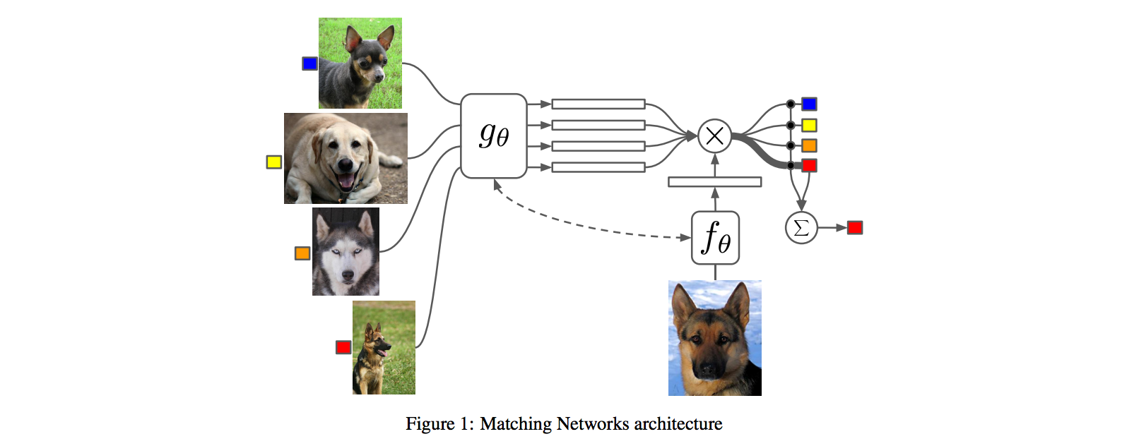![Screen Shot 2016-08-07 at 10.08.44 PM](https://raw.githubusercontent.com/karpathy/paper-notes/master/img/matching_networks/Screen%20Shot%202016-08-07%20at%2010.08.44%20PM.png)

## The training protocol

As the authors amusingly point out in the conclusion (and this is the *duh of course* part), *"one-shot learning is much easier if you train the network to do one-shot learning"*. Therefore, we want the test-time protocol (given N novel classes with only k examples each (e.g. k = 1 or 5), predict new instances to one of N classes) to exactly match the training time protocol.

To create each "episode" of training from a dataset of examples then:

1. Sample a task T from the training data, e.g. select 5 labels, and up to 5 examples per label (i.e. 5-25 examples).
2. To form one episode sample a label set L (e.g. {cats, dogs}) and then use L to sample the support set S and a batch B of examples to evaluate loss on.

The idea on high level is clear but the writing here is a bit unclear on details, of exactly how the sampling is done.

## The model

I find the paper's model description slightly wordy and unclear, but basically we're building a **differentiable nearest neighbor++**. The output \hat{y} for a test example \hat{x} is computed very similar to what you might see in Nearest Neighbors:![Screen Shot 2016-08-07 at 11.14.26 PM](https://raw.githubusercontent.com/karpathy/paper-notes/master/img/matching_networks/Screen%20Shot%202016-08-07%20at%2011.14.26%20PM.png)
where **a** acts as a kernel, computing the extent to which \hat{x} is similar to a training example x_i, and then the labels from the training examples (y_i) are weight-blended together accordingly. The paper doesn't mention this but I assume for classification y_i would presumbly be one-hot vectors.

Now, we're going to embed both the training examples x_i and the test example \hat{x}, and we'll interpret their inner products (or here a cosine similarity) as the "match", and pass that through a softmax to get normalized mixing weights so they add up to 1. No surprises here, this is quite natural:

![Screen Shot 2016-08-07 at 11.20.29 PM](https://raw.githubusercontent.com/karpathy/paper-notes/master/img/matching_networks/Screen%20Shot%202016-08-07%20at%2011.20.29%20PM.png)
Here **c()** is cosine distance, which I presume is implemented by normalizing the two input vectors to have unit L2 norm and taking a dot product. I assume the authors tried skipping the normalization too and it did worse? Anyway, now all that's left to define is the function **f** (i.e. how do we embed the test example into a vector) and the function **g** (i.e. how do we embed each training example into a vector?).

**Embedding the training examples.** This (the function **g**) is a bidirectional LSTM over the examples:

 ![Screen Shot 2016-08-07 at 11.57.10 PM](https://raw.githubusercontent.com/karpathy/paper-notes/master/img/matching_networks/Screen%20Shot%202016-08-07%20at%2011.57.10%20PM.png)

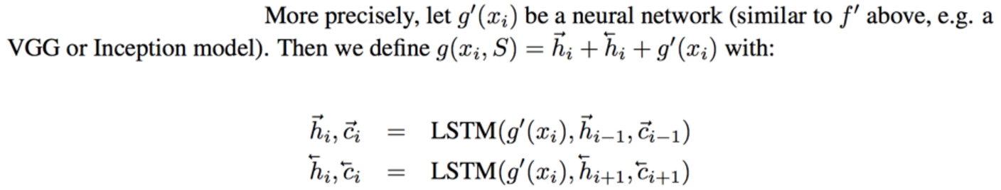
i.e. encoding of i'th example x_i is a function of its "raw" embedding g'(x_i) and the embedding of its friends, communicated through the bidirectional network's hidden states. i.e. each training example is a function of not just itself but all of its friends in the set. This is part of the ++ above, because in a normal nearest neighbor you wouldn't change the representation of an example as a function of the other data points in the training set.

It's odd that the **order** is not mentioned, I assume it's random? This is a bit gross because order matters to a bidirectional LSTM; you'd get different embeddings if you permute the examples. 

**Embedding the test example.** This (the function **f**) is a an LSTM that processes for a fixed amount (K time steps) and at each point also *attends* over the examples in the training set. The encoding is the last hidden state of the LSTM. Again, this way we're allowing the network to change its encoding of the test example as a function of the training examples. Nifty: 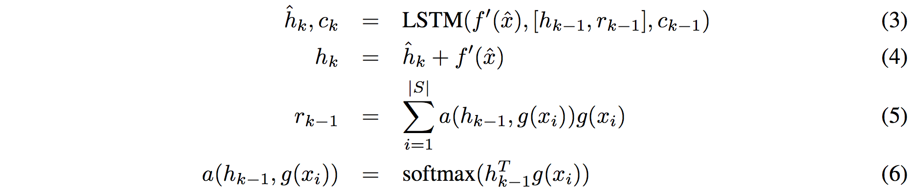![Screen Shot 2016-08-08 at 12.11.15 AM](https://raw.githubusercontent.com/karpathy/paper-notes/master/img/matching_networks/Screen%20Shot%202016-08-08%20at%2012.11.15%20AM.png)

That looks scary at first but it's really just a vanilla LSTM with attention where the input at each time step is constant (f'(\hat{x}), an encoding of the test example all by itself) and the hidden state is a function of previous hidden state but also a concatenated readout vector **r**, which we obtain by attending over the encoded training examples (encoded with **g** from above).

Oh and I assume there is a typo in equation (5), it should say r_k = … without the -1 on LHS. 



## Experiments

**Task**: N-way k-shot learning task. i.e. we're given k (e.g. 1 or 5) labelled examples for N classes that we have not previously trained on and asked to classify new instances into he N classes.

**Baselines:** an "obvious" strategy of using a pretrained ConvNet and doing nearest neighbor based on the codes. An option of finetuning the network on the new examples as well (requires training and careful and strong regularization!).

**MANN** of Santoro et al. [21]: Also a DeepMind paper, a fun NTM-like Meta-Learning approach that is fed a sequence of examples and asked to predict their labels.

**Siamese network** of Koch et al. [11]: A siamese network that takes two examples and predicts whether they are from the same class or not with logistic regression. A test example is labeled with a nearest neighbor: with the class it matches best according to the siamese net (requires iteration over all training examples one by one). Also, this approach is less end-to-end than the one here because it requires the ad-hoc nearest neighbor matching, while here the *exact* end task is optimized for. It's beautiful.



### Omniglot experiments 

### ![Screen Shot 2016-08-08 at 10.21.45 AM](https://github.com/karpathy/paper-notes/raw/master/img/matching_networks/Screen%20Shot%202016-08-08%20at%2010.21.45%20AM.png)

Omniglot of [Lake et al. [14]](http://www.cs.toronto.edu/~rsalakhu/papers/LakeEtAl2015Science.pdf) is a MNIST-like scribbles dataset with 1623 characters with 20 examples each.

Image encoder is a CNN with 4 modules of [3x3 CONV 64 filters, batchnorm, ReLU, 2x2 max pool]. The original image is claimed to be so resized from original 28x28 to 1x1x64, which doesn't make sense because factor of 2 downsampling 4 times is reduction of 16, and 28/16 is a non-integer >1. I'm assuming they use VALID convs?

Results: 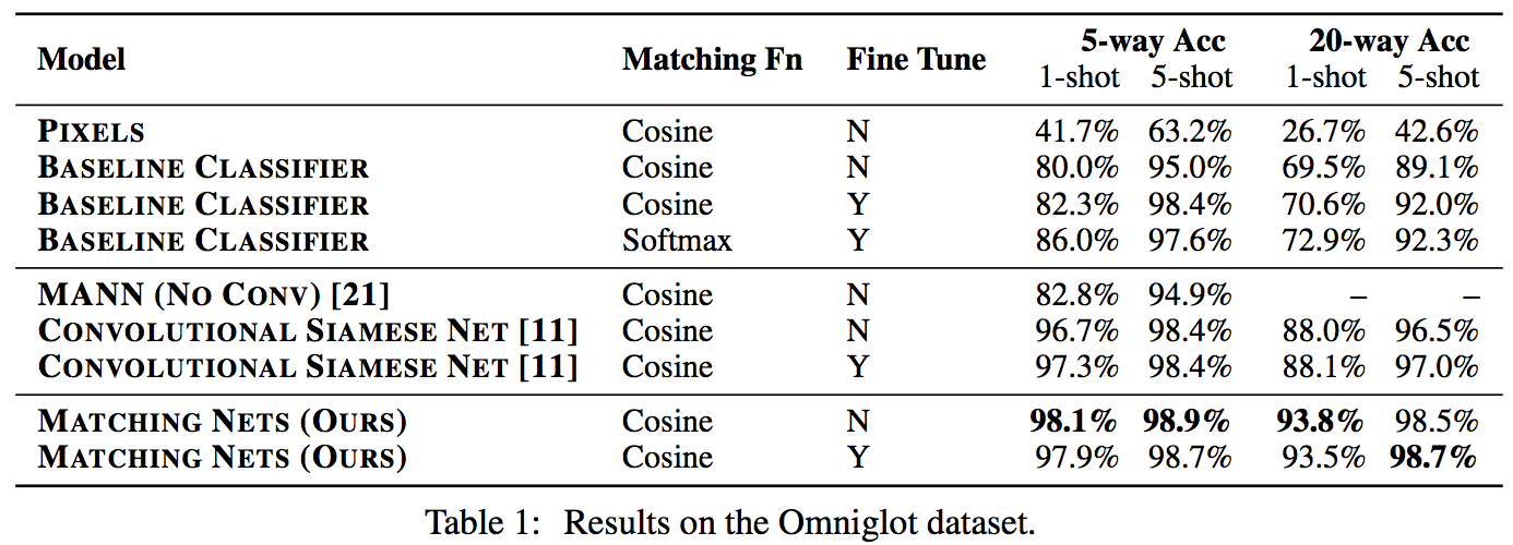![Screen Shot 2016-08-08 at 10.27.46 AM](https://raw.githubusercontent.com/karpathy/paper-notes/master/img/matching_networks/Screen%20Shot%202016-08-08%20at%2010.27.46%20AM.png)

Matching nets do best. Fully Conditional Embeddings (FCE) by which I mean they the "Full Context Embeddings" of Section 2.1.2 instead are not used here, mentioned to not work much better. Finetuning helps a bit on baselines but not with Matching nets (weird).

The comparisons in this table are somewhat confusing:

- I can't find the MANN numbers of 82.8% and 94.9% in their paper [21]; not clear where they come from. E.g. for 5 classes and 5-shot they seem to report 88.4% not 94.9% as seen here. I must be missing something.
- I also can't find the numbers reported here in the Siamese Net [11] paper. As far as I can tell in their Table 2 they report one-shot accuracy, 20-way classification to be 92.0, while here it is listed as 88.1%?
- The results of Lake et al. [14] who proposed Omniglot are also missing from the table. If I'm understanding this correctly they report 95.2% on 1-shot 20-way, while matching nets here show 93.8%, and humans are estimated at 95.5%. That is, the results here appear weaker than those of Lake et al., but one should keep in mind that the method here is significantly more generic and does not make any assumptions about the existence of strokes, etc., and it's a simple, single fully-differentiable blob of neural stuff.

(skipping ImageNet/LM experiments as there are few surprises)

## Conclusions

Good paper, effectively develops a differentiable nearest neighbor trained end-to-end. It's something new, I like it!

A few concerns: 

- A bidirectional LSTMs (not order-invariant compute) is applied over sets of training examples to encode them. The authors don't talk about the order actually used, which presumably is random, or mention this potentially unsatisfying feature. This can be solved by using a recurrent attentional mechanism instead, as the authors are certainly aware of and as has been discussed at length in [ORDER MATTERS: SEQUENCE TO SEQUENCE FOR SETS](https://arxiv.org/abs/1511.06391), where Oriol is also the first author. I wish there was a comment on this point in the paper somewhere.

- The approach also gets quite a bit slower as the number of training examples grow, but once this number is large one would presumable switch over to a parameteric approach.

- It's also potentially concerning that during training the method uses a specific number of examples, e.g. 5-25, so this is the number of that must also be used at test time. What happens if we want the size of our training set to grow online? It appears that we need to retrain the network because the encoder LSTM for the training data is not "used to" seeing inputs of more examples? That is unless you fall back to iteratively subsampling the training data, doing multiple inference passes and averaging, or something like that. If we don't use FCE it can still be that the attention mechanism LSTM can still not be "used to" attending over many more examples, but it's not clear how much this matters. An interesting experiment would be to not use FCE and try to use 100 or 1000 training examples, while only training on up to 25 (with and fithout FCE). Discussion surrounding this point would be interesting.

- Not clear what happened with the Omniglot experiments, with incorrect numbers for [11], [21], and the exclusion of Lake et al. [14] comparison.

- A baseline that is missing would in my opinion also include training of an [Exemplar SVM](https://www.cs.cmu.edu/~tmalisie/projects/iccv11/), which is a much more powerful approach than encode-with-a-cnn-and-nearest-neighbor.

  ​

This paper can be thought as proposing a variational autoencoder applied to a form of meta-learning, i.e. where the input is not a single input but a dataset of inputs. For this, in addition to having to learn an approximate inference network over the latent variable $z_i$ for each input $x_i$ in an input dataset $D$, approximate inference is also learned over a latent variable $c$ that is global to the dataset $D$. By using Gaussian distributions for $z_i$ and $c$, the reparametrization trick can be used to train the variational autoencoder.

The generative model factorizes as

$p(D=(x_1,\dots,x_N), (z_1,\dots,z_N), c) = p(c) \prod_i p(z_i|c) p(x_i|z_i,c)$

and learning is based on the following variational posterior decomposition:

$q((z_1,\dots,z_N), c|D=(x_1,\dots,x_N)) = q(c|D) \prod_i q(z_i|x_i,c)$.

Moreover, latent variable $z_i$ is decomposed into multiple ($L$) layers $z_i = (z_{i,1}, \dots, z_{i,L})$. Each layer in the generative model is directly connected to the input. The layers are generated from $z_{i,L}$ to $z_{i,1}$, each layer being conditioned on the previous (see Figure 1 *Right* for the graphical model), with the approximate posterior following a similar decomposition.

The architecture for the approximate inference network $q(c|D)$ first maps all inputs $x_i\in D$ into a vector representation, then performs mean pooling of these representations to obtain a single vector, followed by a few more layers to produce the parameters of the Gaussian distribution over $c$. 

Training is performed by stochastic gradient descent, over minibatches of datasets (i.e. multiple sets $D$).

The model has multiple applications, explored in the experiments. One is of summarizing a dataset $D$ into a smaller subset $S\in D$. This is done by initializing $S\leftarrow D$ and greedily removing elements of $S$, each time minimizing the KL divergence between $q(c|D)$ and $q(c|S)$ (see the experiments on a synthetic Spatial MNIST problem of section 5.3).

Another application is few-shot classification, where very few examples of a number of classes are given, and a new test example $x'$ must be assigned to one of these classes. Classification is performed by treating the small set of examples of each class $k$ as its own dataset $D_k$. Then, test example $x$ is classified into class $k$ for which the KL divergence between $q(c|x')$ and $q(c|D_k)$ is smallest. Positive results are reported when training on OMNIGLOT classes and testing on either the MNIST classes or unseen OMNIGLOT datasets, when compared to a 1-nearest neighbor classifier based on the raw input or on a representation learned by a regular autoencoder.

Finally, another application is that of generating new samples from an input dataset of examples. The approximate posterior is used to compute $q(c|D)$. Then, $c$ is assigned to its posterior mean, from which a value for the hidden layers $z$ and finally a sample $x$ can be generated. It is shown that this procedure produces convincing samples that are visually similar from those in the input set $D$.

**My two cents**

Another really nice example of deep learning applied to a form of meta-learning, i.e. learning a model that is trained to take *new* datasets as input and generalize even if confronted to datasets coming from an unseen data distribution. I'm particularly impressed by the many tasks explored successfully with the same approach: few-shot classification and generative sampling, as well as a form of summarization (though this last probably isn't really meta-learning). Overall, the approach is quite elegant and appealing.

The very simple, synthetic experiments of section 5.1 and 5.2 are also interesting. Section 5.2 presents the notion of a *prior-interpolation layer*, which is well motivated but seems to be used only in that section. I wonder how important it is, outside of the specific case of section 5.2.

Overall, very excited by this work, which further explores the theme of meta-learning in an interesting way.

**Summary**

Representation (or feature) learning with unsupervised learning has yet really to yield the type of results that many believe to be achievable. For example, we’d like to unleash an unsupervised learning algorithm on all web images and then obtain a representation that captures the various factors of variation we know to be present (e.g. objects and people). One popular approach for this is to train a model that assumes a high-level vector representation with independent components. However, despite a large body of literature on such models by now, such so-called disentangling of these factors of variation still seems beyond our reach.

In this short paper, the authors propose an alternative to this approach. They propose that disentangling might be achievable by learning a representation whose dimensions are each separately **controllable**, i.e. that each have an associated policy which changes the value of that dimension **while letting other dimensions fixed**. 

Specifically, the authors propose to minimize the following objective:

$\mathop{\mathbb{E}}_s\left[\frac{1}{2}||s-g(f(s))||^2_2 \right] - \lambda \sum_k \mathbb{E}_{a,s}\left[\sum_a \pi_k(a|s) \log sel(s,a,k)\right]$

where 
- $s$ is an agent’s state (e.g. frame image) which encoder $f$ and decoder $g$ learn to autoencode
- $k$ iterates over all dimensions of the representation space (output of encoder)
- $a$ iterates over actions that the agent can take
- $\pi_k(a|s)$ is the policy that is meant to control the $k^{\rm th}$ dimension of the representation space $f(s)_k$
- $sel(s,a,k)$ is the selectivity of $f(s)_k$ relative to other dimensions in the representation, at state $s$:

$sel(s,a,k) = \mathop{\mathbb{E}}_{s’\sim {\cal P}_{ss’}^a}\left[\frac{|f_k(s’)-f_k(s)|}{\sum_{k’} |f_{k’}(s’)-f_{k’}(s)| }\right]$

${\cal P}_{ss’}^a$ is the conditional distribution over the next step state $s’$ given that you are at state $s$ and are taking action $a$ (i.e. the environment transition distribution). One can see that selectivity is higher when the change $|f_k(s’)-f_k(s)|$ in dimension $k$ is much larger than the change 
$|f_{k’}(s’)-f_{k’}(s)|$ in the other dimensions $k’$. A directed version of selectivity is also proposed (and I believe was used in the experiments), where the absolute value function is removed and $\log sel$ is replaced with $\log(1+sel)$ in the objective.

The learning objective will thus encourage the discovery of a representation that is informative of the input (in that you can reconstruct it) and for which there exists policies that separately control these dimensions.

Algorithm 1 in the paper describes a learning procedure for optimizing this objective. In brief, for every update, a state $s$ is sampled from which an update for the autoencoder part of the loss can be made. Then, iterating over each dimension $k$, REINFORCE is used to get a gradient estimate of the selectivity part of the loss, to update both the policy $\pi_k$ and the encoder $f$ by using the policy to reach a next state $s’$.

**My two cents**

I find this concept very appealing and thought provoking. Intuitively, I find the idea that valuable features are features which reflect an aspect of our environment that we can control more sensible and possibly less constraining than an assumption of independent features. It also has an interesting analogy of an infant learning about the world by interacting with it.

The caveat is that unfortunately, this concept is currently fairly impractical, since it requires an interactive environment where an agent can perform actions, something we can’t easily have short of deploying a robot with sensors. Moreover, the proposed algorithm seems to assume that each state $s$ is sampled independently for each update, whereas a robot would observe a dependent stream of states. 

Accordingly, the experiments in this short paper are mostly “proof of concept”, on simplistic synthetic environments. Yet they do a good job at illustrating the idea.

To me this means that there’s more interesting work worth doing in what seems to be a promising direction!