**Problem Setting:**

Sequence to Sequence learning (seq2seq) is one of the most successful techniques in machine learning nowadays. The basic idea is to encode a sequence into a vector (or a sequence of vectors if using attention based encoder) and then use a recurrent decoder to decode the target sequence conditioned on the encoder output. While researchers have explored various architectural changes to this basic encoder-decoder model, the standard way of training such seq2seq models is to maximize the likelihood of each successive target word conditioned on the input sequence and the *gold* history of target words. This is also known as *teacher-forcing* in RNN literature. Such an approach has three major issues:

1. **Exposure Bias:** Since we teacher-force the model with *gold* history during training, the model is never exposed to its errors during training. At test time, we will not have access to *gold* history and we feed the history generated by the model. If it is erroneous, the model does not have any clue about how to rectify it.

2. **Loss-Evaluation Mismatch:** While we evaluate the model using sequence level metrics (such as BLEU for Machine Translation), we are training the model with word level cross entropy loss.

3. **Label bias:** Since the word probabilities are normalized at each time step (by using softmax over the final layer of the decoder), this can result in label bias if we vary the number of possible candidates in each step. More about this later. 

**Solution:**

This paper proposes an alternative training procedure for seq2seq models which attempt to solve all the 3 major issues listed above. The idea is to pose seq2seq learning as beam-search optimization problem. Authors begin by removing the final softmax activation function from the decoder. Now instead of probability distributions, we will get score for next possible word. Then the training procedure is changed as follows: At every time step $t$, they maintain a set $S_t$ of $K$ candidate sequences of length $t$. Now the loss function is defined with the following characteristics:

1. If the *gold* sub-sequence of length $t$ is in set $S_t$ and the score for *gold* sub-sequence exceeds the score of the $K$-th ranked candidate by a margin, the model incurs no loss. Now the candidates for next time-step are chosen in a way similar to regular beam-search with beam-size $K$.

2. If the *gold* sub-sequence of length $t$ is in set $S_t$ and it is the $K$-th ranked candidate, then the loss will push the *gold* sequence up by increasing its score. The candidates for next time-step are chosen in a way similar as first case.

3. If the *gold* sub-sequence of length $t$ is NOT in set $S_t$, then the score of the *gold* sequence is increased to be higher than $K$-th ranked candidate by a margin. In this case, candidates for next step or chosen by only considering *gold* word at time $t$ and getting its top-$K$ successors.

4. Further, since we want the full *gold* sequence to be at top of the beam at the end of the search, when $t=T$, the loss is modified to require the score of *gold* sequence to exceed the score of the *highest* ranked incorrect prediction by a margin. 

This non-probabilistic training method has several advantages:

* The model is trained in a similar way it would be tested, since we use beam-search during training as well as testing. Hence this helps to eliminate exposure bias.

* The score based loss can be easily scaled by a mistake-specific cost function. For example, in MT, one could use a cost function which is inversely proportional to BLEU score. So there is no loss-evaluation mismatch.

* Each time step can have different set of successor words based on any hard constraints in the problem. Note that the model is non-probabilistic and hence this varying successor function will not introduce any label bias. Refer [this set of slides][1] for an excellent illustration of label bias.

Cost of forward-prop grows linearly with respect to beam size $K$. However, GPU implementation should help to reduce this cost. Authors propose a clever way of doing BPTT which makes the back-prop almost same cost as ordinary seq2seq training.

**Additional Tricks**

1. Authors pre-train the seq2seq model with regular word level cross-entropy loss and this is crucial since random initialization did not work.

2. Authors use "curriculum beam" strategy in training where they start with beam size of 2 and increase the beam size by 1 for every 2 epochs until it reaches the required beam size. You have to train your model with training beam size of at least test beam size + 1. (i.e $K_{tr} >= K_{te} + 1$).

3. When you use drop-out, you need to be careful to use the same dropout value during back-prop. Authors do this by sharing a single dropout across all sequences in a time step.

**Experiments**

Authors compare the proposed model against basic seq2seq in word ordering, dependency parsing and MT tasks. The proposed model achieves significant improvement over the strong baseline.

**Related Work:**

The whole idea of the paper is based on [learning as search optimization (LaSO) framework][2] of Daume III and Marcu (2005). Other notable related work are training seq2seq models using mix of cross-entropy and REINFORCE called [MIXER][3] and [an actor-critic based seq2seq training][4]. Authors compare with MIXER and they do significantly better than MIXER. 

**My two cents:**

This is one of the important research directions in my opinion. While other recent methods attempt to use reinforcement learning to avoid the issues in word-level cross-entropy training, this paper proposes a really simple score based solution which works very well. While most of the language generation research is stuck with probabilistic framework (I am saying this w.r.t Deep NLP research), this paper highlights the benefits on non-probabilistic generation models. I see this as one potential way of avoiding the nasty scalability issues that come with softmax based generative models.

[1]: http://www.cs.stanford.edu/~nmramesh/crf
[2]: https://www.isi.edu/~marcu/papers/daume05laso.pdf
[3]: http://arxiv.org/pdf/1511.06732v7.pdf
[4]: https://arxiv.org/pdf/1607.07086v2.pdf

In the future, AI and people will work together; hence, we must concern ourselves with ensuring that AI will have interests aligned with our own. 
The authors suggest that it is in our best interests to find a solution to the "value-alignment problem". As recently pointed out by Ian Goodfellow, however,
[this may not always be a good idea](https://www.quora.com/When-do-you-expect-AI-safety-to-become-a-serious-issue).

Cooperative Inverse Reinforcement Learning (CIRL) is a formulation of a cooperative, partial information game between a human and a robot. Both share a reward 
function, but the robot does not initially know what it is. One of the key departures from classical Inverse Reinforcement Learning
is that the teacher, which in this case is the human, is not assumed to act optimally. Rather, it is shown that sub-optimal actions
on the part of the human can result in the robot learning a better reward function. The structure of the CIRL formulation is such that it should encourage the 
human to not attempt to teach by demonstration in a way that greedily maximizes immediate reward. Rather, the human learns how to "best respond" to the robot.

CIRL can be formulated as a dec-POMDP, and reduced to a single-agent POMDP. The authors solved a 2D navigation task with CIRL to demonstrate the inferiority of having the human follow a "demonstration-by-expert" policy as opposed to a "best-response" policy.

Originally posted on my Github [paper-notes](https://github.com/karpathy/paper-notes/blob/master/matching_networks.md) repo.

# Matching Networks for One Shot Learning

By DeepMind crew: **Oriol Vinyals, Charles Blundell, Timothy Lillicrap, Koray Kavukcuoglu, Daan Wierstra**

This is a paper on **one-shot** learning, where we'd like to learn a class based on very few (or indeed, 1) training examples. E.g. it suffices to show a child a single giraffe, not a few hundred thousands before it can recognize more giraffes.

This paper falls into a category of *"duh of course"* kind of paper, something very interesting, powerful, but somehow obvious only in retrospect. I like it.

Suppose you're given a single example of some class and would like to label it in test images.

- **Observation 1**: a standard approach might be to train an Exemplar SVM for this one (or few) examples vs. all the other training examples - i.e. a linear classifier. But this requires optimization.
- **Observation 2:** known non-parameteric alternatives (e.g. k-Nearest Neighbor) don't suffer from this problem. E.g. I could immediately use a Nearest Neighbor to classify the new class without having to do any optimization whatsoever. However, NN is gross because it depends on an (arbitrarily-chosen) metric, e.g. L2 distance. Ew.
- **Core idea**: lets train a fully end-to-end nearest neighbor classifer!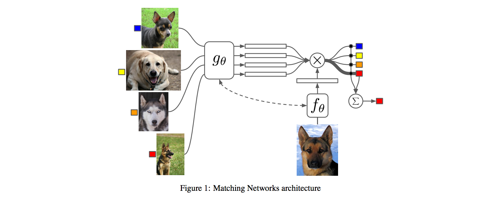![Screen Shot 2016-08-07 at 10.08.44 PM](https://raw.githubusercontent.com/karpathy/paper-notes/master/img/matching_networks/Screen%20Shot%202016-08-07%20at%2010.08.44%20PM.png)

## The training protocol

As the authors amusingly point out in the conclusion (and this is the *duh of course* part), *"one-shot learning is much easier if you train the network to do one-shot learning"*. Therefore, we want the test-time protocol (given N novel classes with only k examples each (e.g. k = 1 or 5), predict new instances to one of N classes) to exactly match the training time protocol.

To create each "episode" of training from a dataset of examples then:

1. Sample a task T from the training data, e.g. select 5 labels, and up to 5 examples per label (i.e. 5-25 examples).
2. To form one episode sample a label set L (e.g. {cats, dogs}) and then use L to sample the support set S and a batch B of examples to evaluate loss on.

The idea on high level is clear but the writing here is a bit unclear on details, of exactly how the sampling is done.

## The model

I find the paper's model description slightly wordy and unclear, but basically we're building a **differentiable nearest neighbor++**. The output \hat{y} for a test example \hat{x} is computed very similar to what you might see in Nearest Neighbors:![Screen Shot 2016-08-07 at 11.14.26 PM](https://raw.githubusercontent.com/karpathy/paper-notes/master/img/matching_networks/Screen%20Shot%202016-08-07%20at%2011.14.26%20PM.png)
where **a** acts as a kernel, computing the extent to which \hat{x} is similar to a training example x_i, and then the labels from the training examples (y_i) are weight-blended together accordingly. The paper doesn't mention this but I assume for classification y_i would presumbly be one-hot vectors.

Now, we're going to embed both the training examples x_i and the test example \hat{x}, and we'll interpret their inner products (or here a cosine similarity) as the "match", and pass that through a softmax to get normalized mixing weights so they add up to 1. No surprises here, this is quite natural:

![Screen Shot 2016-08-07 at 11.20.29 PM](https://raw.githubusercontent.com/karpathy/paper-notes/master/img/matching_networks/Screen%20Shot%202016-08-07%20at%2011.20.29%20PM.png)
Here **c()** is cosine distance, which I presume is implemented by normalizing the two input vectors to have unit L2 norm and taking a dot product. I assume the authors tried skipping the normalization too and it did worse? Anyway, now all that's left to define is the function **f** (i.e. how do we embed the test example into a vector) and the function **g** (i.e. how do we embed each training example into a vector?).

**Embedding the training examples.** This (the function **g**) is a bidirectional LSTM over the examples:

 ![Screen Shot 2016-08-07 at 11.57.10 PM](https://raw.githubusercontent.com/karpathy/paper-notes/master/img/matching_networks/Screen%20Shot%202016-08-07%20at%2011.57.10%20PM.png)

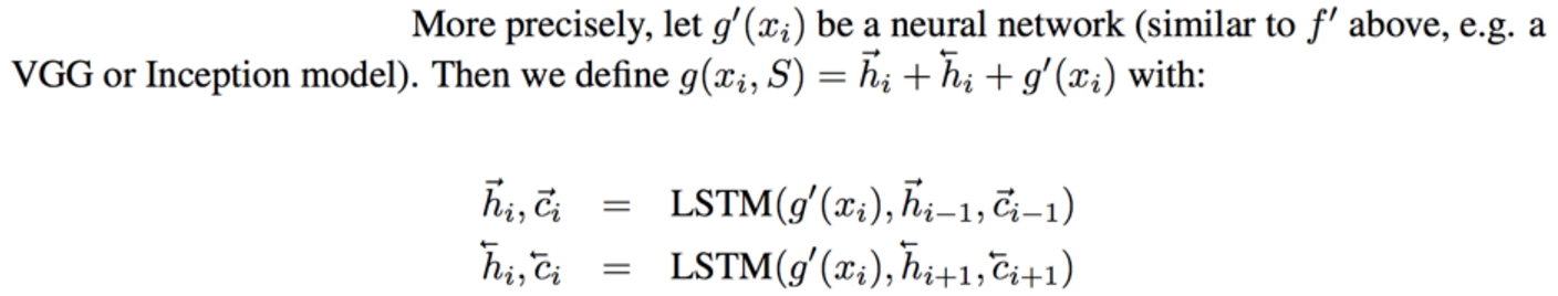
i.e. encoding of i'th example x_i is a function of its "raw" embedding g'(x_i) and the embedding of its friends, communicated through the bidirectional network's hidden states. i.e. each training example is a function of not just itself but all of its friends in the set. This is part of the ++ above, because in a normal nearest neighbor you wouldn't change the representation of an example as a function of the other data points in the training set.

It's odd that the **order** is not mentioned, I assume it's random? This is a bit gross because order matters to a bidirectional LSTM; you'd get different embeddings if you permute the examples. 

**Embedding the test example.** This (the function **f**) is a an LSTM that processes for a fixed amount (K time steps) and at each point also *attends* over the examples in the training set. The encoding is the last hidden state of the LSTM. Again, this way we're allowing the network to change its encoding of the test example as a function of the training examples. Nifty: 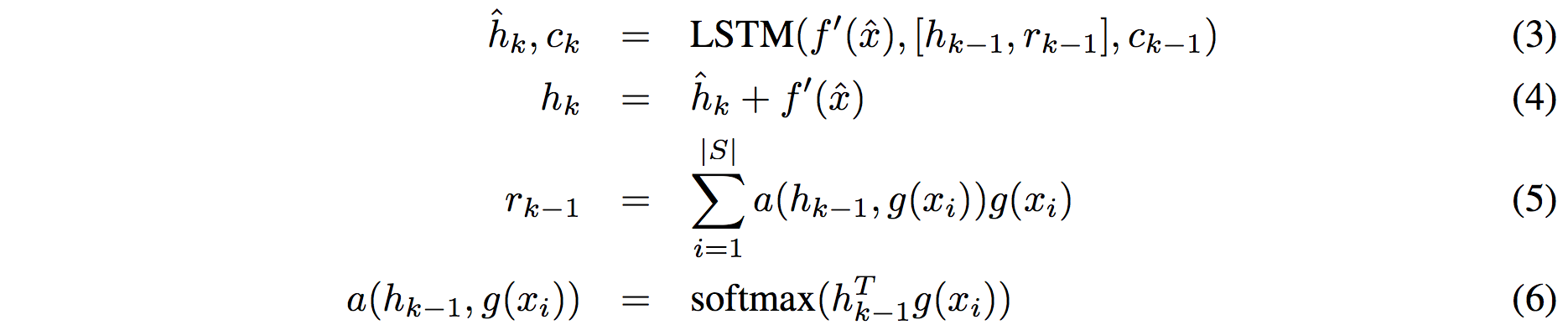![Screen Shot 2016-08-08 at 12.11.15 AM](https://raw.githubusercontent.com/karpathy/paper-notes/master/img/matching_networks/Screen%20Shot%202016-08-08%20at%2012.11.15%20AM.png)

That looks scary at first but it's really just a vanilla LSTM with attention where the input at each time step is constant (f'(\hat{x}), an encoding of the test example all by itself) and the hidden state is a function of previous hidden state but also a concatenated readout vector **r**, which we obtain by attending over the encoded training examples (encoded with **g** from above).

Oh and I assume there is a typo in equation (5), it should say r_k = … without the -1 on LHS. 



## Experiments

**Task**: N-way k-shot learning task. i.e. we're given k (e.g. 1 or 5) labelled examples for N classes that we have not previously trained on and asked to classify new instances into he N classes.

**Baselines:** an "obvious" strategy of using a pretrained ConvNet and doing nearest neighbor based on the codes. An option of finetuning the network on the new examples as well (requires training and careful and strong regularization!).

**MANN** of Santoro et al. [21]: Also a DeepMind paper, a fun NTM-like Meta-Learning approach that is fed a sequence of examples and asked to predict their labels.

**Siamese network** of Koch et al. [11]: A siamese network that takes two examples and predicts whether they are from the same class or not with logistic regression. A test example is labeled with a nearest neighbor: with the class it matches best according to the siamese net (requires iteration over all training examples one by one). Also, this approach is less end-to-end than the one here because it requires the ad-hoc nearest neighbor matching, while here the *exact* end task is optimized for. It's beautiful.



### Omniglot experiments 

### ![Screen Shot 2016-08-08 at 10.21.45 AM](https://github.com/karpathy/paper-notes/raw/master/img/matching_networks/Screen%20Shot%202016-08-08%20at%2010.21.45%20AM.png)

Omniglot of [Lake et al. [14]](http://www.cs.toronto.edu/~rsalakhu/papers/LakeEtAl2015Science.pdf) is a MNIST-like scribbles dataset with 1623 characters with 20 examples each.

Image encoder is a CNN with 4 modules of [3x3 CONV 64 filters, batchnorm, ReLU, 2x2 max pool]. The original image is claimed to be so resized from original 28x28 to 1x1x64, which doesn't make sense because factor of 2 downsampling 4 times is reduction of 16, and 28/16 is a non-integer >1. I'm assuming they use VALID convs?

Results: 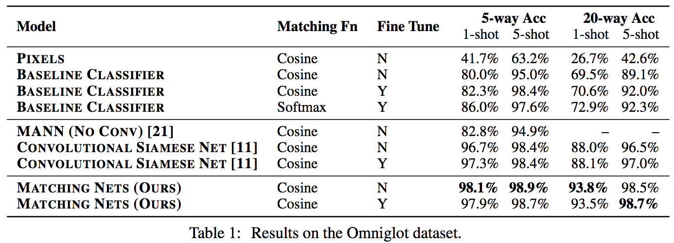![Screen Shot 2016-08-08 at 10.27.46 AM](https://raw.githubusercontent.com/karpathy/paper-notes/master/img/matching_networks/Screen%20Shot%202016-08-08%20at%2010.27.46%20AM.png)

Matching nets do best. Fully Conditional Embeddings (FCE) by which I mean they the "Full Context Embeddings" of Section 2.1.2 instead are not used here, mentioned to not work much better. Finetuning helps a bit on baselines but not with Matching nets (weird).

The comparisons in this table are somewhat confusing:

- I can't find the MANN numbers of 82.8% and 94.9% in their paper [21]; not clear where they come from. E.g. for 5 classes and 5-shot they seem to report 88.4% not 94.9% as seen here. I must be missing something.
- I also can't find the numbers reported here in the Siamese Net [11] paper. As far as I can tell in their Table 2 they report one-shot accuracy, 20-way classification to be 92.0, while here it is listed as 88.1%?
- The results of Lake et al. [14] who proposed Omniglot are also missing from the table. If I'm understanding this correctly they report 95.2% on 1-shot 20-way, while matching nets here show 93.8%, and humans are estimated at 95.5%. That is, the results here appear weaker than those of Lake et al., but one should keep in mind that the method here is significantly more generic and does not make any assumptions about the existence of strokes, etc., and it's a simple, single fully-differentiable blob of neural stuff.

(skipping ImageNet/LM experiments as there are few surprises)

## Conclusions

Good paper, effectively develops a differentiable nearest neighbor trained end-to-end. It's something new, I like it!

A few concerns: 

- A bidirectional LSTMs (not order-invariant compute) is applied over sets of training examples to encode them. The authors don't talk about the order actually used, which presumably is random, or mention this potentially unsatisfying feature. This can be solved by using a recurrent attentional mechanism instead, as the authors are certainly aware of and as has been discussed at length in [ORDER MATTERS: SEQUENCE TO SEQUENCE FOR SETS](https://arxiv.org/abs/1511.06391), where Oriol is also the first author. I wish there was a comment on this point in the paper somewhere.

- The approach also gets quite a bit slower as the number of training examples grow, but once this number is large one would presumable switch over to a parameteric approach.

- It's also potentially concerning that during training the method uses a specific number of examples, e.g. 5-25, so this is the number of that must also be used at test time. What happens if we want the size of our training set to grow online? It appears that we need to retrain the network because the encoder LSTM for the training data is not "used to" seeing inputs of more examples? That is unless you fall back to iteratively subsampling the training data, doing multiple inference passes and averaging, or something like that. If we don't use FCE it can still be that the attention mechanism LSTM can still not be "used to" attending over many more examples, but it's not clear how much this matters. An interesting experiment would be to not use FCE and try to use 100 or 1000 training examples, while only training on up to 25 (with and fithout FCE). Discussion surrounding this point would be interesting.

- Not clear what happened with the Omniglot experiments, with incorrect numbers for [11], [21], and the exclusion of Lake et al. [14] comparison.

- A baseline that is missing would in my opinion also include training of an [Exemplar SVM](https://www.cs.cmu.edu/~tmalisie/projects/iccv11/), which is a much more powerful approach than encode-with-a-cnn-and-nearest-neighbor.

  ​

This paper describes how rank pooling, a very recent approach for pooling representations organized in a sequence $\\{{\bf v}_t\\}_{t=1}^T$, can be used in an end-to-end trained neural network architecture.

Rank pooling is an alternative to average and max pooling for sequences, but with the distinctive advantage of maintaining some order information from the sequence. Rank pooling first solves a regularized (linear) support vector regression (SVR) problem where the inputs are the vector representations ${\bf v}_t$ in the sequence and the target is the corresponding index $t$ of that representation in the sequence (see Equation 5). The output of rank pooling is then simply the linear regression parameters $\bf{u}$ learned for that sequence. Because of the way ${\bf u}$ is trained, we can see that ${\bf u}$ will capture order information, as successful training would imply that ${\bf u}^\top {\bf v}_t < {\bf u}^\top {\bf v}_{t'} $ if $t < t'$. See [this paper](https://www.robots.ox.ac.uk/~vgg/rg/papers/videoDarwin.pdf) for more on rank pooling.

While previous work has focused on using rank pooling on hand-designed and fixed representations, this paper proposes to use ConvNet features (pre-trained on ImageNet) for the representation and backpropagate through rank pooling to fine-tune the ConvNet features. Since the output of rank pooling corresponds to an argmin operation, passing gradients through this operation is not as straightforward as for average or max pooling. However, it turns out that if the objective being minimized (in our case regularized SVR) is twice differentiable, gradients with respect to its argmin can be computed (see Lemmas 1 and 2). The authors derive the gradient for rank pooling (Equation 21). Finally, since its gradient requires inverting a matrix (corresponding to a hessian), the authors propose to either use an efficient procedure for computing it by exploiting properties of sums of rank-one matrices (see Lemma 3) or to simply use an approximation based on using a diagonal hessian.

In experiments on two small scale video activity recognition datasets (UCF-Sports and Hollywood2), the authors show that fine-tuning the ConvNet features significantly improves the performance of rank pooling and makes it superior to max and average pooling.

**My two cents**

This paper was eye opening for me, first because I did not realize that one could backpropagate through an operation corresponding to an argmin that doesn't have a closed form solution (though apparently this paper isn't the first to make that observation). Moreover, I did not know about rank pooling, which itself is a really thought provoking approach to pooling representations in a way that preserves some organizational information about the original representations.

I wonder how sensitive the results are to the value of the regularization constant of the SVR problem. The authors mention some theoretical guaranties on the stability of the solution found by SVR in general, but intuitively I would expect that the regularization constant would play a large role in the stability.

I'll be looking forward to any future attempts to increase the speed of rank pooling (or any similar method). Indeed, as the authors mention, it is currently too slow to be used on the larger video datasets that are currently available. 

Code for computing rank pooling (though not for computing its gradients) seems to be available [here](https://bitbucket.org/bfernando/videodarwin).

This paper poses the the problem of querying a large corpus of aerial video as a subgraph matching problem. Here the video data has been transformed into a large graph where each frame contains labeled objects such as person, object, or car which become nodes and then the edges are relationships such as time (between sequential video frames) and distance (in current frame and in future frames). 

The reason the graph is built is to we can query it with graphs that represent what we are looking for. The first example in the paper (below) shows an example query (called $Q$). This query asks to "Find a person near an object then after some time or distance they are still near and there is a car". 

![](http://i.imgur.com/6AKVCYX.png)

The goal now is to find the most similar subgraphs in the larger graph. The game here is to reduce the complexity of the search into something that is not as bad as the subgraph isomorphism problem. Even though this is worse because we what things that are similar and not necessarily exact to the query.

They filter the larger graph (that represents the video) into a smaller graph that only includes nodes and edges that can match those in the query graph (This graph is called the coarse graph $C$). Another is to filter the query $Q$ into a smaller graph $T$ which retains nodes and edges that have the most discriminative power.

### WORK IN PROGRESS