Strong consistency increases latency; weak consistency is hard to reason about. Compromising between the two, a number of databases allow each operation to run with either strong or weak consistency. Ideally, users choose the minimal set of strongly consistent operations needed to enforce some application specific invariant. However, deciding which operations to run with strong consistency and which to run with weak consistency can be very challenging. This paper

 - introduces a formal hybrid consistency model which subsumes many existing consistency models,
 - introduces a modular proof rule which can determine whether a given consistency model enforces an invariant, and
 - implements a prototype using a standard SMT solver.

Consistency Model, Informally. Consider

 - a set of states $s, s_{init} \in$ State,
 - a set of operations Op = {o, ...},
 - a set of values $\bot$ in Val, and
 - a set of replicas $r_1, r_2,$ ....

The denotation of an operation is denoted F_o where

 - F_o: State -> (Val x (State -> State)),
 - F_o^val(s) = F_o(s)[0] (the value returned by the operation), and
 - F_o^eff(s) = F_o(s)[1] (the effect of the operation).

For example, a banking operation may let states range over natural numbers where

 - F_deposit_a(s) = (\bot, fun s' -> s' + a)
 - F_interest(s) = (\bot, fun s' -> s' + 0.05 * s)
 - F_query(s) = (s, fun s' -> s')

If all operations commute (i.e. forall o1, o2, s1, s2. F_o1(s1) o F_o2(s2) = F_o2(s2) o F_o1(s1)), then all replicas are guaranteed to converge. However, convergence does not guarantee all application invariants are maintained. For example, an invariant I = {s | s >= 0} could be violated by merging concurrent withdrawals. To enforce invariants, we introduce a token system which can be used to order certain operations.

A token system TS = (Token, #) is a set of tokens Token and a symmetric relation # over Token. We say two sets of tokens T1 # T2 if exists t1 in T1, t2 in T2. t1 # t2. We also update our definition of operations to acquire tokens:

 - F_o: State -> (Val x (State -> State) x P(Token)),
 - F_o^val(s) = F_o(s)[0] (the value returned by the operation),
 - F_o^eff(s) = F_o(s)[1] (the effect of the operation), and
 - F_o^tok(s) = F_o(s)[2] (the tokens acquired by the operation).

Our consistency model will ensure that two operations that acquire conflicting operations will be ordered.

Formal Semantics. Recall a strict partial order is a partial order that is transitive and irreflexive (e.g. sets ordered by strict subset). Given a partial order R, we say (a, b) \in R or a -R-> b. Consider a countably infinite set Event of events ranged over by e, f, g. If operations are like transactions, an event is like applying a transaction at a replica.

- Definition 1. Given token system TS = (Token, #), an execution is a tuple X = (E, oper, rval, tok, hb) where
   - E \subset Event is a finite subset of events,
   - oper: E -> Op designates the operation of each event,
   - rval: E -> Val designates the return value of each event,
   - tok: E -> P(Token) designates the tokens acquired by each event, and
   - hb \subset Event x Event is a happens before strict partial order where forall e, f. tok(e) # tok(f) => (e-hb->f or f-hb->e).

An execution formalizes operations executing at various replicas concurrently, and the happens before relation captures how these operations are propagated between replicas. The transitivity of the happens before relation ensures at least causal consistency.

Let

 - Exec(TS) be the set of all executions over token system TS, and
 - ctxt(e, X) = (E, X.oper|E, X.rval|E, X.tok|E, X.hb|E) be the context of e where E = X.hb^-1(e). Intuitively, ctxt(e, X) is the subexection of X that only includes operations causally preceding e.

Executions are directed graphs of operations, but without a semantics, they are rather meaningless. Here, we define a relation evald_F \subset Exec(TS) x P(State) where evald_F(Y) is the set of all final states Y can be in after all operations are propagated to all replicas. We'll see shortly that if all non-token-conflicting operations commute, then evald_F is a function.

 - evald_F(Y) = {} if Y.E = {}, and
 - evald_F(Y) = {F_e^eff(s)(s') | e \in max(Y), s \in evald_F(ctxt(e, Y)), s' \in evalfd_F(Y|Y.E - {e})} otherwise.

Now

 - Definition 2. An execution X \in Exec(TS) is consistent with TS and F denoted X |= TS, F if forall e \in X.e. exists s \in evald_F(ctxt(e, x)). X.val(e) = F_X.oper(e)^val(s) and X.tok(e = F_X.oper(e)^tok(s)).

We let Exec(TS, F) = {X | X |= TS, F}. Consistent operations are closed under context. Furthermore, evald_F is a function when restricted to consistent executions where non-token-conflicting operations commute. We call this function eval_F.

This model can model a number of consistency models:

 - Causal consistency. Let Token = {}.
 - Sequential consistency. Let Token = {t}, t # t, and F_o^tok(s) = {t} for all o.
 - RedBlue Consistency. Let Token = {t}, t # t, and F_o^tok(s) = {t} for all red o and F_o^tok(s) = {} for all blue o.

State Based Proof Rule. We want to construct a proof rule to establish the fact that Exec(TS, F) \subset eval_F^-1(I). That is, every execution results in a state that satisfies the invariant. Since executions are closed under context, this also means that all operations execute on a state that satisfies the invariant.

Our proof rule involves a guarantee relation G(t) over states which describes all possible state changes that can occur while holding token t. Similarly, G_0 describes the state transitions that can occur without holding any tokens.

Here is the proof rule.

 - S1: s_init \in I.
 - S2: G_0(I) \subset I and forall t. G(t)(I) \subset I.
 - S3: forall o, s, s'.
    - s \in I and
    - (s, s') \in (G_0 \cup G(F_o^tok(s)^\bot))* =>
    - (s', F_o^eff(s)(s')) \in G_0 \cup G(F_o^tok(s)).


In English,

 - S1: s_init satisfies the invariant.
 - S2: G and G_0 preserve the invariant.
 - S3: If we start in any state s that satisfies the invariant and can transition in any finite number of steps to any state s' without acquiring any tokens conflicting with o, then we can transition from s' to F_o^eff(s)(s') in a single step using the tokens acquired by o.

Event Based Proof Rule and Soundness. Instead of looking at states, we can instead look at executions. That is, if we let invariants I \subset Exec(TS), then we want to write a proof rule to ensure Exec(TS, F) \subset I. That is, all consistent executions satisfy the invariant. Again, we use a guarantee G \subset Exec(TS) x Exec(TS).

 - E1: X_init \in I.
 - E2: G(I) \in I.
 - E3: forall X, X', X''. forall e in X''.E.
    - X'' |= TS, F and
    - X' = X''|X''.E - {e} and
    - e \in max(X'') and
    - X = ctxt(e, X'') and
    - X \in I and
    - (X, X') \in G* =>
    - (X', X'') \in G.

This proof rule is proven sound. The event based rule and its soundness is derived from this.

Examples and Automation. The authors have built a banking, auction, and courseware application in this style. They have also built a prototype that you give TS, F, and I and it determines if Exec(T, f) \subset eval_F^-1(I). Their prototype modifies the state-based proof rule eliminating the transitive closure and introducing intermediate predicates.

## **Introduction**
This paper presents a novel interactive tool for efficient and reproducible boundary extraction with minimal user input. Despite the user not being very accurate with the manual marking of the seed points, the algorithm snaps the boundary to the nearest strong object edge. Unlike active contour models where the user is unaware of how the final boundary will look like after energy minimization (which, if unsatisfactory, requires the entire process to be repeated again), this algorithm is interactive and therefore the user is aware of the "live-wire boundary snapping". Moreover, "boundary cooling" and "on-the-fly training" are two novel contributions of the paper which help reduce user input while maintaining the stability of the boundary.

## **Method**
Modeling the boundary detection problem as a graph search, the new objective is to find the optimal path between a start node (pixel) to a goal node (pixel), where the total cost of any path is the sum of the local costs of the path. Let the local cost of a directed edge from pixel ${p}$ to a neighboring pixel ${q}$ be
$$
    l({p}, {q}) = \underbrace{0.43f_Z({q})}_{\text{Laplacian zero crossing}} + \underbrace{0.43f_G({q})}_{\text{gradient magnitude}} + \underbrace{0.14f_D({p}, {q})}_{\text{gradient direction}}
$$
where the weights have been empirically chosen by the authors.

The gradient magnitude $f_G({g})$ needs to be a term so that higher image gradients will correspond to lower costs in order to provide a "first-order" positioning of the live wire boundary. As such, the gradient magnitude G is defined as

$$
    f_G = 1 - \frac{G}{max(G)}
$$
The Laplacian zero crossing term is a binary edge feature and acts as a "second order" fine tuning term for boundary localization.

$$
  f_Z({q}) = \left\{
  \begin{array}{@{}ll@{}}
    0, & \text{if}\ I_L({q}) = 0 \: or \: a \: neighbor \: with \: opposite \: sign \\
    1, & \text{otherwise} \\
  \end{array}\right.
$$
where $I_L$ represents the convolution of the image with a Laplacian edge operator.

The gradient direction term is associated with penalizing sharp changes in the boundary direction and therefore effectively adds a boundary smoothness constraint.

Let ${D(p)}$ be the unit vector normal to the image gradient at pixel ${p}$. Then the gradient direction cost can be represented as:
$$
    f_D({p}, {q}) = \frac{2}{3\pi}\big\{cos[d_p(({p}, {q})]^{-1} + cos[d_q(({p}, {q})]^{-1}\big\}
$$ where
$$
    d_p(({p}, {q}) = {D(p).L(p,q)}
    $$$$
    d_p(({p}, {q}) = {L(p,q).D(q)}, \: and \text{} \\ 
    $$$$
      {L(p,q)} = \left\{
      \begin{array}{@{}ll@{}}
        {q-p}, & \text{if}\ {D(p).(q-p)} \geq 0 \\
        {p-q}, & \text{otherwise} \\
      \end{array}\right.
$$
where ${L(p,q)}$ represents the normalized the bidirectional edge between pixels ${p}$ and ${q}$ and represents the direction of the link between them so that the difference between ${p}$ and this direction is minimized. Intuitively, this cost is low when the gradient direction of the two pixels are similar to each other and the link between them.

Starting at a user-selected seed point, the boundary finding is continued in the direction of the minimum cumulative cost, which creates a dynamic 'wavefront' along the directions to highest interest (which happen to be along the edges). For a path length of $n$, the boundary growing requires $n$ iterations, which is significantly more efficient than the previously used approaches.

A distribution of a variety of features (such as the image gradient $f_G$ weighted with a monotonically decreasing function (either linear or Gaussian) determines the contribution of each of the closest $t$ pixels, and the algorithm follows the edge of current interest (rather than the strongest) and associates lower costs with current edge features and higher costs for edge features not belonging to the current edge, thereby performing a dynamic or "on-the-fly" training.

The algorithm also exhibits what the paper calls "data-driven path cooling" - as the cursor (and therefore the free point) moves further away from the seed point, progressively longer portions of the boundary become fixed and only the new parts of the boundary need to be updated.

## **Results and Discussion**
Using the algorithm, the boundaries are extracted in one-fifth of the time required for manually tracing the boundary, while doing so with a 4.4x higher accuracy and 4.8x higher reproducibility. However, the paper admits that boundary detection can be difficult with objects with "hair like boundaries". Moreover, this technique cannot be extended to N-dimensional images.

TLDR; The authors show that we can improve the performance of a reference task (like translation) by simultaneously training other tasks, like image caption generation or parsing, and vice versa. The authors evaluate 3 MLT (Multi-Task Learning) scenarios: One-to-many, many-to-one and many-to-many. The authors also find that using skip-thought unsupervised training works well for improving translation performance, but sequence autoencoders don't.

#### Key Points

- 4-Layer seq2seq LSTM, 1000-dimensional cells each layer and embedding, batch size 128, dropout 0.2, SGD wit LR 0.7 and decay.
- The authors define a mixing ratio for parameter updates that is defined with respect to a reference tasks. Picking the right mixing ratio is a hyperparameter.
- One-To-Many experiments: Translation (EN -> GER) + Parsing (EN). Improves result for both tasks. Surprising that even a very small amount of parsing updates significantly improves MT result.
- Many-to-One experiments: Captioning + Translation (GER -> EN). Improves result for both tasks (wrt. to reference task)
- Many-to-Many experiments: Translation (EN <-> GER) + Autoencoders or Skip-Thought. Skip-Thought vectors improve the result, but autoencoders make it worse.
- No attention mechanism


#### Questions / Notes

- I think this is very promising work. it may allow us to build general-purpose systems for many tasks, even those that are not strictly seq2seq. We can easily substitute classification.
- How do the authors pick the mixing ratios for the parameter updates, and how sensitive are the results to these ratios? It's a new hyperparameter and I would've liked to see graphs for these. Makes me wonder if they picked "just the right" ratio to make their results look good, or if these architectures are robust.
- The authors found that seq2seq autoencoders don't improve translation, but skip-thought does. In fact, autoencoders made translation performance significantly worse. That's very surprising to me. Is there any intuition behind that? 

The paper introduced the famous MapReduce paradigm and created a huge impact in the BigData world. Many systems including Hadoop MapReduce and Spark were developed along the lines of the paradigm described in the paper. MapReduce was conceptualized to handle cases where computation to be performed was straightforward but parallelizing the computation and taking care of other aspects of distributed computing was a pain.

A MapReduce computation takes as input a set of key/value pairs and outputs another set of key/value pairs. The computation consists of 2 parts:

1. Map — A function to process input key/value pairs to generate a set of intermediate key/value pairs. All the values corresponding to each intermediate key are grouped together and sent over to the Reduce function.
2. Reduce — A function that merges all the intermediate values associated with the same intermediate key.

The Map/Reduce primitives are inspired by similar primitives defined in Lisp and other functional programming languages.

A program written in MapReduce is automatically parallelized without the programmer having to care about the underlying details of partitioning the input data, scheduling the computations or handling failures. The paper mentions many interesting applications like distributed grep, inverted index and distributed sort which can be expressed by MapReduce logic.

#### Execution Overview
When MapReduce function is invoked, following steps take place:

1. The input data is partitioned into a set of M splits of equal size.
2. One of the nodes in the cluster becomes the master and rest become the workers. There are M Map and R Reduce tasks.
3. The Map invocations are distributed across multiple machines containing the input partitions.
4. Each worker reads the content of the partition and applies the Map function to it. Intermediate results are buffered in memory and periodically written back to local disk.
5. The locations are passed on to the master which passes it on to reduce workers. These workers read the intermediate data and sort it.
6. Reduce worker iterates over the sorted data and for each unique intermediate key, passes the key and intermediate values to Reduce function. The output is appended to an output file.
7. Once all map and reduce tasks are over, the control is returned to the user program.

As we saw, the map phase is divided into M tasks and reduce phase into R tasks. Keeping M and R much larger than the number of nodes helps to improve dynamic load balancing and speeds up failure recovery. But since the master has to make O(M+R) scheduling decisions and keep O(M*R) states in memory, the value of M and R can not be arbitrarily large.

#### Master Node
The master maintains the state of each map-reduce task and the identity of each worker machine. The location of the intermediate file also moves between the map and reduce operations via the master. The master pings each worker periodically. In case, it does not her back, it marks the worker as failed and assigns its task to some other worker. If a map task fails, all the reduce workers are notified about the newly assigned worker. Master failure results in computation termination in which case the client may choose to restart the computation.

#### Locality
MapReduce takes advantage of the fact that input data is stored on the machines performing the computations. The master tries to schedule a map job on a machine that contains the corresponding input data. Thus, most of the data is read locally and network IO is saved. This locality optimization is inspired by active disks where computation is pushed to processing elements close to the disk.

#### Backup Tasks
Stragglers are machines that take an unusually long time to complete one of the last few Map or Reduce tasks and can increase the overall execution time of the program. To account for these, when a MapReduce operation is close to completion, the master schedules backup executions of remaining in-progress tasks. This may lead to some redundant computation but can help to reduce the start-to-end execution time.

#### Refinements
MapReduce supports a variety of refinements including:
1. Users can specify an optional combiner function that performs a partial merge over the data before sending it over the network. This combiner operation would be performed after the Map function and would reduce the amount of data to be sent over the network.
2. MapReduce can be configured to detect if certain records fail deterministically and skip those records. It is very useful in scenarios where a few missing records can be tolerated.
3. Within a given partition, the intermediate key/value pairs are guaranteed to be processed in increasing key order.
4. Side-effect is supported in the sense that MapReduce tasks can produce auxiliary files as additional outputs from their operation.
5. MapReduce can be run in sequential mode on the local machine to facilitate debugging and profiling.
6. The master runs an internal HTTP Server that exports status pages showing metadata of computation and links to output and error files.
7. MapReduce provides a counter facility to keep track of occurrence of various events like the number of documents processed. Counters like the number of key-value pairs processed are tracked by default.

Other refinements include custom partitioning function and support for different input/output types.

MapReduce was profiled for two computations(grep and sort) running on a large cluster of commodity machines. The results were very solid. The grep program scanned ten billion records in 150 seconds and the sort program could sort ten billion records in 891 seconds (including the startup overhead). Moreover, the profiling showed the benefit of backup tasks and that the system is resilient to node failure.
Other than performance, MapReduce offers many more benefits. The user code tends to be small and understandable as the code taking care of the distributed aspect is now abstracted. So the user does not have to worry about issues like machine failure and networking error. Moreover the system can be easily scaled horizontally. Lastly, the performance is good enough that conceptually unrelated computations can be maintained separately instead of having to mix every thing together in the name of saving that extra pass over the data.

  * They present a model which adds color to grayscale images (e.g. to old black and white images).
  * It works best with 224x224 images, but can handle other sizes too.

### How
  * Their model has three feature extraction components:
    * Low level features:
      * Receives 1xHxW images and outputs 512xH/8xW/8 matrices.
      * Uses 6 convolutional layers (3x3, strided, ReLU) for that.
    * Global features:
      * Receives the low level features and converts them to 256 dimensional vectors.
      * Uses 4 convolutional layers (3x3, strided, ReLU) and 3 fully connected layers (1024 -> 512 -> 256; ReLU) for that.
    * Mid-level features:
      * Receives the low level features and converts them to 256xH/8xW/8 matrices.
      * Uses 2 convolutional layers (3x3, ReLU) for that.
  * The global and mid-level features are then merged with a Fusion Layer.
    * The Fusion Layer is basically an extended convolutional layer.
    * It takes the mid-level features (256xH/8xW/8) and the global features (256) as input and outputs a matrix of shape 256xH/8xW/8.
    * It mostly operates like a normal convolutional layer on the mid-level features. However, its weight matrix is extended to also include weights for the global features (which will be added at every pixel).
    * So they use something like `fusion at pixel u,v = sigmoid(bias + weights * [global features, mid-level features at pixel u,v])` - and that with 256 different weight matrices and biases for 256 filters.
  * After the Fusion Layer they use another network to create the coloring:
    * This network receives 256xH/8xW/8 matrices (merge of global and mid-level features) and generates 2xHxW outputs (color in L\*a\*b\* color space).
    * It uses a few convolutional layers combined with layers that do nearest neighbour upsampling.
  * The loss for the colorization network is a MSE based on the true coloring.
  * They train the global feature extraction also on the true class labels of the used images.
  * Their model can handle any sized image. If the image doesn't have a size of 224x224, it must be resized to 224x224 for the gobal feature extraction. The mid-level feature extraction only uses convolutions, therefore it can work with any image size. 

### Results
  * The training set that they use is the "Places scene dataset".
  * After cleanup the dataset contains 2.3M training images (205 different classes) and 19k validation images.
  * Users rate images colored by their method in 92.6% of all cases as real-looking (ground truth: 97.2%).
  * If they exclude global features from their method, they only achieve 70% real-looking images.
  * They can also extract the global features from image A and then use them on image B. That transfers the style from A to B. But it only works well on semantically similar images.

![Architecture](https://raw.githubusercontent.com/aleju/papers/master/neural-nets/images/Let_there_be_Color__architecture.png?raw=true "Architecture")

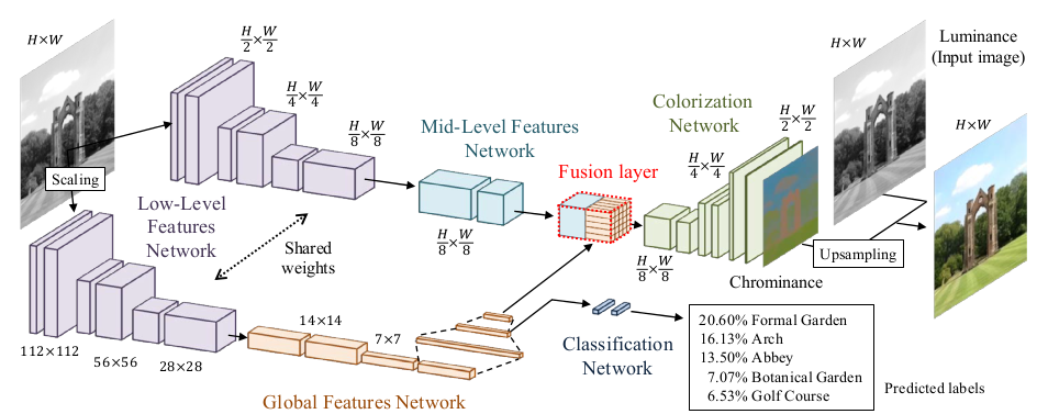
*Architecture of their model.*


![Old images](https://raw.githubusercontent.com/aleju/papers/master/neural-nets/images/Let_there_be_Color__old_images.png?raw=true "Old images")

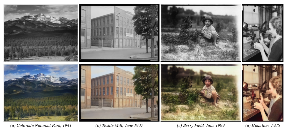
*Their model applied to old images.*

--------------------

# Rough chapter-wise notes

* (1) Introduction
  * They use a CNN to color images.
  * Their network extracts global priors and local features from grayscale images.
  * Global priors:
    * Extracted from the whole image (e.g. time of day, indoor or outdoors, ...).
    * They use class labels of images to train those. (Not needed during test.)
  * Local features: Extracted from small patches (e.g. texture).
  * They don't generate a full RGB image, instead they generate the chrominance map using the CIE L\*a\*b\* colorspace.
  * Components of the model:
    * Low level features network: Generated first.
    * Mid level features network: Generated based on the low level features.
    * Global features network: Generated based on the low level features.
    * Colorization network: Receives mid level and global features, which were merged in a fusion layer.
  * Their network can process images of arbitrary size.
  * Global features can be generated based on another image to change the style of colorization, e.g. to change the seasonal colors from spring to summer.

* (3) Joint Global and Local Model
  * <repetition of parts of the introduction>
  * They mostly use ReLUs.
  * (3.1) Deep Networks
    * <standard neural net introduction>
  * (3.2) Fusing Global and Local Features for Colorization
    * Global features are used as priors for local features.
    * (3.2.1) Shared Low-Level Features
      * The low level features are which's (low level) features are fed into the networks of both the global and the medium level features extractors.
      * They generate them from the input image using a ConvNet with 6 layers (3x3, 1x1 padding, strided/no pooling, ends in 512xH/8xW/8).
    * (3.2.2) Global Image Features
      * They process the low level features via another network into global features.
      * That network has 4 conv-layers (3x3, 2 strided layers, all 512 filters), followed by 3 fully connected layers (1024, 512, 256).
      * Input size (of low level features) is expected to be 224x224.
    * (3.2.3) Mid-Level Features
      * Takes the low level features (512xH/8xW/8) and uses 2 conv layers (3x3) to transform them to 256xH/8xW/8.
    * (3.2.4) Fusing Global and Local Features
      * The Fusion Layer is basically an extended convolutional layer.
      * It takes the mid-level features (256xH/8xW/8) and the global features (256) as input and outputs a matrix of shape 256xH/8xW/8.
      * It mostly operates like a normal convolutional layer on the mid-level features. However, its weight matrix is extended to also include weights for the global features (which will be added at every pixel).
      * So they use something like `fusion at pixel u,v = sigmoid(bias + weights * [global features, mid-level features at pixel u,v])` - and that with 256 different weight matrices and biases for 256 filters.
    * (3.2.5) Colorization Network
      * The colorization network receives the 256xH/8xW/8 matrix from the fusion layer and transforms it to the 2xHxW chrominance map.
      * It basically uses two upsampling blocks, each starting with a nearest neighbour upsampling layer, followed by 2 3x3 convs.
      * The last layer uses a sigmoid activation.
      * The network ends in a MSE.
  * (3.3) Colorization with Classification
    * To make training more effective, they train parts of the global features network via image class labels.
    * I.e. they take the output of the 2nd fully connected layer (at the end of the global network), add one small hidden layer after it, followed by a sigmoid output layer (size equals number of class labels).
    * They train that with cross entropy. So their global loss becomes something like `L = MSE(color accuracy) + alpha*CrossEntropy(class labels accuracy)`.
  * (3.4) Optimization and Learning
    * Low level feature extraction uses only convs, so they can be extracted from any image size.
    * Global feature extraction uses fc layers, so they can only be extracted from 224x224 images.
    * If an image has a size unequal to 224x224, it must be (1) resized to 224x224, fed through low level feature extraction, then fed through the global feature extraction and (2) separately (without resize) fed through the low level feature extraction and then fed through the mid-level feature extraction.
    * However, they only trained on 224x224 images (for efficiency).
    * Augmentation: 224x224 crops from 256x256 images; random horizontal flips.
    * They use Adadelta, because they don't want to set learning rates. (Why not adagrad/adam/...?)

* (4) Experimental Results and Discussion
  * They set the alpha in their loss to `1/300`.
  * They use the "Places scene dataset". They filter images with low color variance (including grayscale images). They end up with 2.3M training images and 19k validation images. They have 205 classes.
  * Batch size: 128.
  * They train for about 11 epochs.
  * (4.1) Colorization results
    * Good looking colorization results on the Places scene dataset.
  * (4.2) Comparison with State of the Art
    * Their method succeeds where other methods fail.
    * Their method can handle very different kinds of images.
  * (4.3) User study
    * When rated by users, 92.6% think that their coloring is real (ground truth: 97.2%).
    * Note: Users were told to only look briefly at the images.
  * (4.4) Importance of Global Features
    * Their model *without* global features only achieves 70% user rating.
    * There are too many ambiguities on the local level.
  * (4.5) Style Transfer through Global Features
    * They can perform style transfer by extracting the global features of image B and using them for image A.
  * (4.6) Colorizing the past
    * Their model performs well on old images despite the artifacts commonly found on those.
  * (4.7) Classification Results
    * Their method achieves nearly as high classification accuracy as VGG (see classification loss for global features).
  * (4.8) Comparison of Color Spaces
    * L\*a\*b\* color space performs slightly better than RGB and YUV, so they picked that color space.
  * (4.9) Computation Time
    * One image is usually processed within seconds.
    * CPU takes roughly 5x longer.
  * (4.10) Limitations and Discussion
    * Their approach is data driven, i.e. can only deal well with types of images that appeared in the dataset.
    * Style transfer works only really well for semantically similar images.
    * Style transfer cannot necessarily transfer specific colors, because the whole model only sees the grayscale version of the image.
    * Their model tends to strongly prefer the most common color for objects (e.g. grass always green).