[link]
Summary by Alexander Jung 8 years ago
* They describe a model for human pose estimation, i.e. one that finds the joints ("skeleton") of a person in an image.
* They argue that part of their model resembles a Markov Random Field (but in reality its implemented as just one big neural network).
### How
* They have two components in their network:
* Part-Detector:
* Finds candidate locations for human joints in an image.
* Pretty standard ConvNet. A few convolutional layers with pooling and ReLUs.
* They use two branches: A fine and a coarse one. Both branches have practically the same architecture (convolutions, pooling etc.). The coarse one however receives the image downscaled by a factor of 2 (half width/height) and upscales it by a factor of 2 at the end of the branch.
* At the end they merge the results of both branches with more convolutions.
* The output of this model are 4 heatmaps (one per joint? unclear), each having lower resolution than the original image.
* Spatial-Model:
* Takes the results of the part detector and tries to remove all detections that were false positives.
* They derive their architecture from a fully connected Markov Random Field which would be solved with one step of belief propagation.
* They use large convolutions (128x128) to resemble the "fully connected" part.
* They initialize the weights of the convolutions with joint positions gathered from the training set.
* The convolutions are followed by log(), element-wise additions and exp() to resemble an energy function.
* The end result are the input heatmaps, but cleaned up.
### Results
* Beats all previous models (with and without spatial model).
* Accuracy seems to be around 90% (with enough (16px) tolerance in pixel distance from ground truth).
* Adding the spatial model adds a few percentage points of accuracy.
* Using two branches instead of one (in the part detector) adds a bit of accuracy. Adding a third branch adds a tiny bit more.
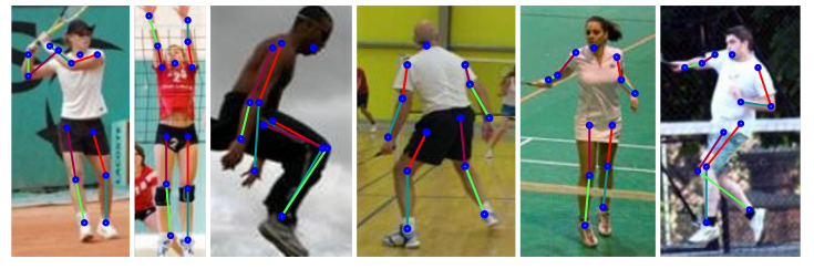
*Example results.*
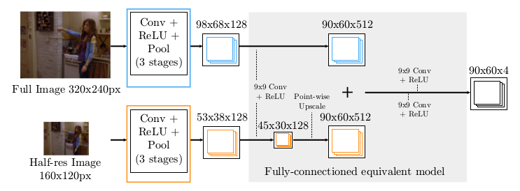
*Part Detector network.*
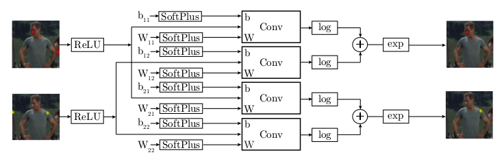
*Spatial Model (apparently only for two input heatmaps).*
-------------------------
# Rough chapter-wise notes
* (1) Introduction
* Human Pose Estimation (HPE) from RGB images is difficult due to the high dimensionality of the input.
* Approaches:
* Deformable-part models: Traditionally based on hand-crafted features.
* Deep-learning based disciminative models: Recently outperformed other models. However, it is hard to incorporate priors (e.g. possible joint- inter-connectivity) into the model.
* They combine:
* A part-detector (ConvNet, utilizes multi-resolution feature representation with overlapping receptive fields)
* Part-based Spatial-Model (approximates loopy belief propagation)
* They backpropagate through the spatial model and then the part-detector.
* (3) Model
* (3.1) Convolutional Network Part-Detector
* This model locates possible positions of human key joints in the image ("part detector").
* Input: RGB image.
* Output: 4 heatmaps, one per key joint (per pixel: likelihood).
* They use a fully convolutional network.
* They argue that applying convolutions to every pixel is similar to moving a sliding window over the image.
* They use two receptive field sizes for their "sliding window": A large but coarse/blurry one, a small but fine one.
* To implement that, they use two branches. Both branches are mostly identical (convolutions, poolings, ReLU). They simply feed a downscaled (half width/height) version of the input image into the coarser branch. At the end they upscale the coarser branch once and then merge both branches.
* After the merge they apply 9x9 convolutions and then 1x1 convolutions to get it down to 4xHxW (H=60, W=90 where expected input was H=320, W=240).
* (3.2) Higher-level Spatial-Model
* This model takes the detected joint positions (heatmaps) and tries to remove those that are probably false positives.
* It is a ConvNet, which tries to emulate (1) a Markov Random Field and (2) solving that MRF approximately via one step of belief propagation.
* The raw MRF formula would be something like `<likelihood of joint A per px> = normalize( <product over joint v from joints V> <probability of joint A per px given a> * <probability of joint v at px?> + someBiasTerm)`.
* They treat the probabilities as energies and remove from the formula the partition function (`normalize`) for various reasons (e.g. because they are only interested in the maximum value anyways).
* They use exp() in combination with log() to replace the product with a sum.
* They apply SoftPlus and ReLU so that the energies are always positive (and therefore play well with log).
* Apparently `<probability of joint v at px?>` are the input heatmaps of the part detector.
* Apparently `<probability of joint A per px given a>` is implemented as the weights of a convolution.
* Apparently `someBiasTerm` is implemented as the bias of a convolution.
* The convolutions that they use are large (128x128) to emulate a fully connected graph.
* They initialize the convolution weights based on histograms gathered from the dataset (empirical distribution of joint displacements).
* (3.3) Unified Models
* They combine the part-based model and the spatial model to a single one.
* They first train only the part-based model, then only the spatial model, then both.
* (4) Results
* Used datasets: FLIC (4k training images, 1k test, mostly front-facing and standing poses), FLIC-plus (17k, 1k ?), extended-LSP (10k, 1k).
* FLIC contains images showing multiple persons with only one being annotated. So for FLIC they add a heatmap of the annotated body torso to the input (i.e. the part-detector does not have to search for the person any more).
* The evaluation metric roughly measures, how often predicted joint positions are within a certain radius of the true joint positions.
* Their model performs significantly better than competing models (on both FLIC and LSP).
* Accuracy seems to be at around 80%-95% per joint (when choosing high enough evaluation tolerance, i.e. 10px+).
* Adding the spatial model to the part detector increases the accuracy by around 10-15 percentage points.
* Training the part detector and the spatial model jointly adds ~3 percentage points accuracy over training them separately.
* Adding the second filter bank (coarser branch in the part detector) adds around 5 percentage points accuracy. Adding a third filter bank adds a tiny bit more accuracy.


