* They use an implementation of Q-learning (i.e. reinforcement learning) with CNNs to automatically play Atari games.
  * The algorithm receives the raw pixels as its input and has to choose buttons to press as its output. No hand-engineered features are used. So the model "sees" the game and "uses" the controller, just like a human player would.
  * The model achieves good results on various games, beating all previous techniques and sometimes even surpassing human players.

### How
  * Deep Q Learning
    * *This is yet another explanation of deep Q learning, see also [this blog post](http://www.nervanasys.com/demystifying-deep-reinforcement-learning/) for longer explanation.*
    * While playing, sequences of the form (`state1`, `action1`, `reward`, `state2`) are generated.
      * `state1` is the current game state. The agent only sees the pixels of that state. (Example: Screen shows enemy.)
      * `action1` is an action that the agent chooses. (Example: Shoot!)
      * `reward` is the direct reward received for picking `action1` in `state1`. (Example: +1 for a kill.)
      * `state2` is the next game state, after the action was chosen in `state1`. (Example: Screen shows dead enemy.)
    * One can pick actions at random for some time to generate lots of such tuples. That leads to a replay memory.
    * Direct reward
      * After playing randomly for some time, one can train a model to predict the direct reward given a screen (we don't want to use the whole state, just the pixels) and an action, i.e. `Q(screen, action) -> direct reward`.
      * That function would need a forward pass for each possible action that we could take. So for e.g. 8 buttons that would be 8 forward passes. To make things more efficient, we can let the model directly predict the direct reward for each available action, e.g. for 3 buttons `Q(screen) -> (direct reward of action1, direct reward of action2, direct reward of action3)`.
      * We can then sample examples from our replay memory. The input per example is the screen. The output is the reward as a tuple. E.g. if we picked button 1 of 3 in one example and received a reward of +1 then our output/label for that example would be `(1, 0, 0)`.
      * We can then train the model by playing completely randomly for some time, then sample some batches and train using a mean squared error. Then play a bit less randomly, i.e. start to use the action which the network thinks would generate the highest reward. Then train again, and so on.
    * Indirect reward
      * Doing the previous steps, the model will learn to anticipate the *direct* reward correctly. However, we also want it to predict indirect rewards. Otherwise, the model e.g. would never learn to shoot rockets at enemies, because the reward from killing an enemy would come many frames later.
      * To learn the indirect reward, one simply adds the reward value of highest reward action according to `Q(state2)` to the direct reward.
      * I.e. if we have a tuple (`state1`, `action1`, `reward`, `state2`), we would not add (`state1`, `action1`, `reward`) to the replay memory, but instead (`state1`, `action1`, `reward + highestReward(Q(screen2))`). (Where `highestReward()` returns the reward of the action with the highest reward according to Q().)
      * By training to predict `reward + highestReward(Q(screen2))` the network learns to anticipate the direct reward *and* the indirect reward. It takes a leap of faith to accept that this will ever converge to a good solution, but it does.
      * We then add `gamma` to the equation: `reward + gamma*highestReward(Q(screen2))`. `gamma` may be set to 0.9. It is a discount factor that devalues future states, e.g. because the world is not deterministic and therefore we can't exactly predict what's going to happen. Note that Q will automatically learn to stack it, e.g. `state3` will be discounted to `gamma^2` at `state1`.
  * This paper
    * They use the mentioned Deep Q Learning to train their model Q.
    * They use a k-th frame technique, i.e. they let the model decide upon an action at (here) every 4th frame.
    * Q is implemented via a neural net. It receives 84x84x4 grayscale pixels that show the game and projects that onto the rewards of 4 to 18 actions.
    * The input is HxWx4 because they actually feed the last 4 frames into the network, instead of just 1 frame. So the network knows more about what things are moving how.
    * The network architecture is:
      * 84x84x4 (input)
      * 16 convs, 8x8, stride 4, ReLU
      * 32 convs, 4x4, stride 2, ReLU
      * 256 fully connected neurons, ReLU
      * <N_actions> fully connected neurons, linear
    * They use a replay memory of 1 million frames.

### Results
  * They ran experiments on the Atari games Beam Rider, Breakout, Enduro, Pong, Qbert, Seaquest and Space Invaders.
  * Same architecture and hyperparameters for all games.
  * Rewards were based on score changes in the games, i.e. they used +1 (score increases) and -1 (score decreased).
  * Optimizer: RMSProp, Batch Size: 32.
  * Trained for 10 million examples/frames per game.
  * They had no problems with instability and their average Q value per game increased smoothly.
  * Their method beats all other state of the art methods.
  * They managed to beat a human player in games that required not so much "long" term strategies (the less frames the better).
  * Video: starts at 46:05. 
 https://youtu.be/dV80NAlEins?t=46m05s 


![Algorithm](https://raw.githubusercontent.com/aleju/papers/master/neural-nets/images/Playing_Atari_with_Deep_Reinforcement_Learning__algorithm.png?raw=true "Algorithm")

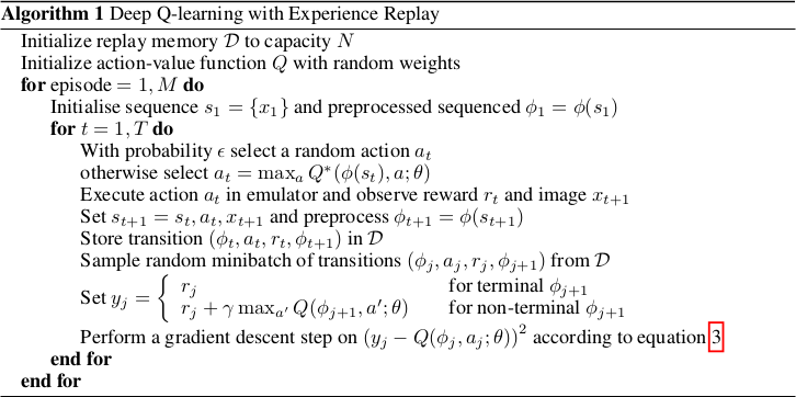
*The original full algorithm, as shown in the paper.*

--------------------

### Rough chapter-wise notes

* (1) Introduction
  * Problems when using neural nets in reinforcement learning (RL):
    * Reward signal is often sparse, noise and delayed.
    * Often assumption that data samples are independent, while they are correlated in RL.
    * Data distribution can change when the algorithm learns new behaviours.
  * They use Q-learning with a CNN and stochastic gradient descent.
  * They use an experience replay mechanism (i.e. memory) from which they can sample previous transitions (for training).
  * They apply their method to Atari 2600 games in the Arcade Learning Environment (ALE).
  * They use only the visible pixels as input to the network, i.e. no manual feature extraction.

* (2) Background
  * blablabla, standard deep q learning explanation

* (3) Related Work
  * TD-Backgammon: "Solved" backgammon. Worked similarly to Q-learning and used a multi-layer perceptron.
  * Attempts to copy TD-Backgammon to other games failed.
  * Research was focused on linear function approximators as there were problems with non-linear ones diverging.
  * Recently again interest in using neural nets for reinforcement learning. Some attempts to fix divergence problems with gradient temporal-difference methods.
  * NFQ is a very similar method (to the one in this paper), but worked on the whole batch instead of minibatches, making it slow. It also first applied dimensionality reduction via autoencoders on the images instead of training on them end-to-end.
  * HyperNEAT was applied to Atari games and evolved a neural net for each game. The networks learned to exploit design flaws.

* (4) Deep Reinforcement Learning
  * They want to connect a reinforcement learning algorithm with a deep neural network, e.g. to get rid of handcrafted features.
  * The network is supposes to run on the raw RGB images.
  * They use experience replay, i.e. store tuples of (pixels, chosen action, received reward) in a memory and use that during training.
  * They use Q-learning.
  * They use an epsilon-greedy policy.
  * Advantages from using experience replay instead of learning "live" during game playing:
    * Experiences can be reused many times (more efficient).
    * Samples are less correlated.
    * Learned parameters from one batch don't determine as much the distributions of the examples in the next batch.
  * They save the last N experiences and sample uniformly from them during training.
  * (4.1) Preprocessing and Model Architecture
    * Raw Atari images are 210x160 pixels with 128 possible colors.
    * They downsample them to 110x84 pixels and then crop the 84x84 playing area out of them.
    * They also convert the images to grayscale.
    * They use the last 4 frames as input and stack them.
    * So their network input has shape 84x84x4.
    * They use one output neuron per possible action. So they can compute the Q-value (expected reward) of each action with one forward pass.
    * Architecture: 84x84x4 (input) => 16 8x8 convs, stride 4, ReLU => 32 4x4 convs stride 2 ReLU => fc 256, ReLU => fc N actions, linear
    * 4 to 18 actions/outputs (depends on the game).
    * Aside from the outputs, the architecture is the same for all games.

* (5) Experiments
  * Games that they played: Beam Rider, Breakout, Enduro, Pong, Qbert, Seaquest, Space Invaders
  * They use the same architecture und hyperparameters for all games.
  * They give a reward of +1 whenever the in-game score increases and -1 whenever it decreases.
  * They use RMSProp.
  * Mini batch size was 32.
  * They train for 10 million frames/examples.
  * They initialize epsilon (in their epsilon greedy strategy) to 1.0 and decrease it linearly to 0.1 at one million frames.
  * They let the agent decide upon an action at every 4th in-game frame (3rd in space invaders).
  * (5.1) Training and stability
    * They plot the average reward und Q-value per N games to evaluate the agent's training progress,
    * The average reward increases in a noisy way.
    * The average Q value increases smoothly.
    * They did not experience any divergence issues during their training.
  * (5.2) Visualizating the Value Function
    * The agent learns to predict the value function accurately, even for rather long sequences (here: ~25 frames).
  * (5.3) Main Evaluation
    * They compare to three other methods that use hand-engineered features and/or use the pixel data combined with significant prior knownledge.
    * They mostly outperform the other methods.
    * They managed to beat a human player in three games. The ones where the human won seemed to require strategies that stretched over longer time frames.

The paper introduces two key properties of deep neural networks:

- Semantic meaning of individual units.
    - Earlier works analyzed learnt semantics by finding images that maximally activate individual units.
    - Authors observe that there is no difference between individual units and random linear combinations of units.
    - It is the entire space of activations that contains the bulk of semantic information.

- Stability of neural networks to small perturbations in input space.
    - Networks that generalize well are expected to be robust to small perturbations in the input, i.e. imperceptible noise in the input shouldn't change the predicted class.
    - Authors find that networks can be made to misclassify an image by applying a certain imperceptible perturbation, which is found by maximizing the network's prediction error.
    - These 'adversarial examples' generalize well to different architectures trained on different data subsets.

## Strengths

- The authors propose a way to make networks more robust to small perturbations by training them with adversarial examples in an adaptive manner, i.e. keep changing the pool of adversarial examples during training. In this regard, they draw a connection with hard-negative mining, and a network trained with adversarial examples performs better than others.

- Formal description of how to generate adversarial examples and mathematical analysis of a network's stability to perturbations are useful studies.

## Weaknesses / Notes

- Two images that are visually indistinguishable to humans but classified differently by the network is indeed an intriguing observation.

- The paper feels a little half-baked in parts, and some ideas could've been presented more clearly.

The paper discusses and empirically investigates by empirical testing the effect of "catastrophic forgetting" (**CF**), i.e. the inability of a model to perform a task it was previously trained to perform if retrained to perform a second task. 

An illuminating example is what happens in ML systems with convex objectives: regardless of the initialization (i.e. of what was learnt by doing the first task), the training of the second task will always end in the global minimum, thus totally "forgetting" the first one. 

Neuroscientific evidence (and common sense) suggest that the outcome of the experiment is deeply influenced by the similarity of the tasks involved. Namely, if (i) the two tasks are *functionally identical but input is presented in a different format* or if (ii)  *tasks are similar* and the third case for (iii) *dissimilar tasks*. 

Relevant examples may be provided respectively by (i) performing the same image classification task starting from two different image representations as RGB or HSL, (ii) performing image classification tasks with semantically similar as classifying two similar animals and (iii) performing a text classification followed by image classification. 

The problem is investigated by an empirical study covering two methods of training ("SGD" and "dropout") combined with 4 activations functions (logistic sigmoid, RELU, LWTA, Maxout). A random search is carried out on these parameters. 

From a practitioner's point of view, it is interesting to note that dropout has been set to 0.5 in hidden units and 0.2 in the visible one since this is a reasonably well-known parameter. 

## Why the paper is important
It is apparently the first to provide a systematic empirical analysis of CF. Establishes a framework and baselines to face the problem.

## Key conclusions, takeaways and modelling remarks
* dropout helps in preventing CF
* dropout seems to increase the optimal model size with respect to the model without dropout 
* choice of activation function has a less consistent effect than dropout\no dropout choice
* dissimilar task experiment provides a  notable exception of then dissimilar task experiment
* the previous hypothesis that LWTA activation is particularly resistant to CF is rejected  (even if it performs best in the new task in the dissimilar task pair the behaviour is inconsistent)
* choice of activation function should always be cross-validated
* If computational resources are insufficient for cross-validation the combination dropout + maxout activation function is recommended.

#### Introduction

* Open-domain Question Answering (Open QA) - efficiently querying large-scale knowledge base(KB) using natural language.
* Two main approaches:
    * Information Retrieval
        * Transform question (in natural language) into a valid query(in terms of KB) to get a broad set of candidate answers.
        * Perform fine-grained detection on candidate answers.
    * Semantic Parsing
        * Interpret the correct meaning of the question and convert it into an exact query.
* Limitations:
    * Human intervention to create lexicon, grammar, and schema.
* This work builds upon the previous work where an embedding model learns low dimensional vector representation of words and symbols.
* [Link](https://arxiv.org/abs/1406.3676) to the paper.

#### Task Definition

* Input - Training set of questions (paired with answers).
* KB providing a structure among the answers.
* Answers are entities in KB and questions are strings with one identified KB entity.
* The paper has used FREEBASE as the KB.
* Datasets
    * WebQuestions - Built using FREEBASE, Google Suggest API, and Mechanical Turk.
    * FREEBASE triplets transformed into questions.
    * Clue Web Extractions dataset with entities linked with FREEBASE triplets.
    * Dataset of paraphrased questions using WIKIANSWERS.

#### Embedding Questions and Answers

* Model learns low-dimensional vector embeddings of words in question entities and relation types of FREEBASE such that questions and their answers are represented close to each other in the joint embedding space.
* Scoring function $S(q, a)$, where $q$ is a question and $a$ is an answer, generates high score if $a$ answers $q$.
    * $S(q, a) = f(q)^{T} . g(a)$
    * $f(q)$ maps question to embedding space. 
    * $f(q) = W \phi (q)$
    * $W$ is a matrix of dimension $K * N$
    * $K$ - dimension of embedding space (hyper parameter).
    * $N$ - total number of words/entities/relation types.
    * $\psi(q)$ - Sparse Vector encoding the number of times a word appears in $q$.
* Similarly, $g(a) = W \psi (a)$ maps answer to embedding space.
* $\psi(a)$ gives answer representation, as discussed below.

#### Possible Representations of Candidate Answers

* Answer represented as a **single entity** from FREEBASE and TBD is a one-of-N encoded vector.
* Answer represented as a **path** from question to answer. The paper considers only one or two hop paths resulting in 3-of-N or 4-of-N encoded vectors(middle entities are not recorded).
* Encode the above two representations using **subgraph representation** which represents both the path and the entire subgraph of entities connected to answer entity as a subgraph. Two embedding representations are used to differentiate between entities in path and entities in the subgraph.
* SubGraph approach is based on the hypothesis that including more information about the answers would improve results.

#### Training and Loss Function

* Minimize margin based ranking loss to learn matrix $W$.
* Stochastic Gradient Descent, multi-threaded with Hogwild.

#### Multitask Training of Embeddings

* To account for a large number of synthetically generated questions, the paper also multi-tasks the training of model with paraphrased prediction.
* Scoring function $S_{prp} (q1, q2) = f(q1)^{T} f(q2)$, where $f$ uses the same weight matrix $W$ as before.
* High score is assigned if $q1$ and $q2$ belong to same paraphrase cluster.
* Additionally, the model multitasks the task of mapping embeddings of FREEBASE entities (mids) to actual words.

#### Inference

* For each question, a candidate set is generated.
* The answer (from candidate set) with the highest set is reported as the correct answer.
* Candidate set generation strategy
    * $C_1$ - All KB triplets containing the KB entity from the question forms a candidate set. Answers would be limited to 1-hop paths.
    * $C_2$ - Rank all relation types and keep top 10 types and add only those 2-hop candidates where the selected relations appear in the path.
    
#### Results

* $C_2$ strategy outperforms $C_1$ approach supporting the hypothesis that a richer representation for answers can store more information.
* Proposed approach outperforms the baseline methods but is outperformed by an ensemble of proposed approach with semantic parsing via paraphrasing model.

Spatial Pyramid Pooling (SPP) is a technique which allows Convolutional Neural Networks (CNNs) to use input images of any size, not only $224\text{px} \times 224\text{px}$ as most architectures do. (However, there is a lower bound for the size of the input image).

## Idea

* Convolutional layers operate on any size, but fully connected layers need fixed-size inputs
* Solution:
  * Add a new SPP layer on top of the last convolutional layer, before the fully connected layer
  * Use an approach similar to bag of words (BoW), but maintain the spatial information. The BoW approach is used for text classification, where the order of the words is discarded and only the number of occurences is kept.
  * The SPP layer operates on each feature map independently.
  * The output of the SPP layer is of dimension $k \cdot M$, where $k$ is the number of feature maps the SPP layer got as input and $M$ is the number of bins.

Example: We could use spatial pyramid pooling with 21 bins:

* 1 bin which is the max of the complete feature map
* 4 bins which divide the image into 4 regions of equal size (depending on the input size) and rectangular shape. Each bin gets the max of its region.
* 16 bins which divide the image into 4 regions of equal size (depending on the input size) and rectangular shape. Each bin gets the max of its region.

## Evaluation

* Pascal VOC 2007, Caltech101: state-of-the-art, without finetuning
* ImageNet 2012: Boosts accuracy for various CNN architectures
* ImageNet Large Scale Visual Recognition Challenge (ILSVRC) 2014: Rank #2


## Code

The paper claims that the code is [here](http://research.microsoft.com/en-us/um/people/kahe/), but this seems not to be the case any more.

People have tried to implement it with Tensorflow ([1](http://stackoverflow.com/q/40913794/562769), [2](https://github.com/fchollet/keras/issues/2080), [3](https://github.com/tensorflow/tensorflow/issues/6011)), but by now no public working implementation is available.


## Related papers

* [Atrous Convolution](https://arxiv.org/abs/1606.00915)