[link]
Summary by inFERENCe 9 years ago
I spend the week at ICML, and this paper on generative models is one of my favourites so far:
To be clear: this post doesn't add much to the presentation of the paper, but I will attempt to summarise my understanding of it. Also, I want to make clear that this is not my work.
Unsupervised learning has been one of the most interesting areas of machine learning in the last decades, but it is in the spotlight again since the deep learning crowd started to care about it. Unsupervised learning is hard because evaluating the loss function people want to use (log likelihood) is intractable for most interesting models. Therefore people come up with
- alternative objective functions, such as adversarial training, maximum mean discrepancy, or pseudolikelihood, which can be evaluated for a large class of interesting models
- alternative optimisation methods or approximate inference methods such as contrastive divergence or variational Bayes
- models that have some nice properties. This paper is an example of the latter
#### The key idea behind the paper
What we typically try to do in representation learning is to map data to a latent representation. While the Data can have arbitrarily complex distribution along some complicated nonlinear manifold, we want the computed latent representations to have a nice distribution, like a multivariate Gaussian.
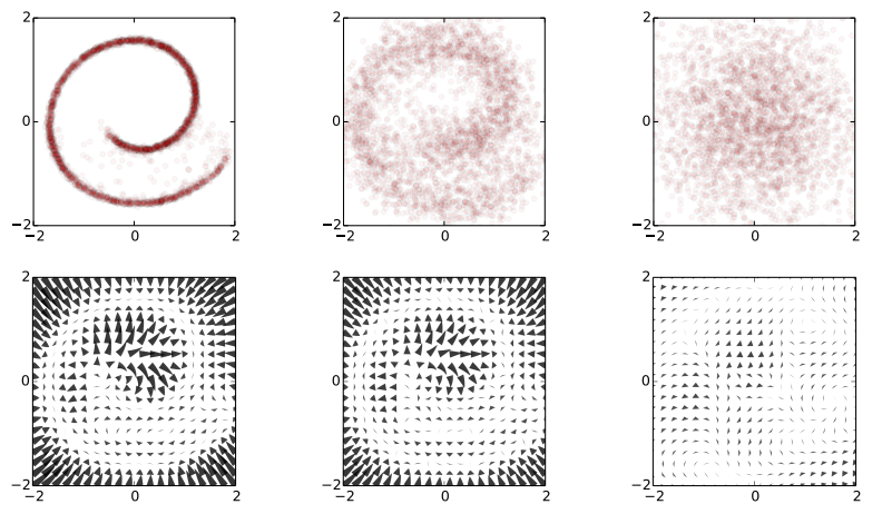
This paper takes this idea very explicitly using a stochastic mapping to turn data into a representation: a random diffusion process. If you take any data, and apply Brownian motion-like stochastic process to this, you will end up with a standard Gaussian distributed variable, due to the stationarity of the Brownian motion. Below image shows an example: 2D observations (left) have a complex data distribution along the Swiss roll manifold. If one applies Brownian motion to each datapoint, the complicated structure starts to diffuse, and eventually the data is scrambled to become white noise (right).

Now the trick the authors used is to train a dynamical system to inverts this random walk, to be able to reconstruct the original data distribution from the random Gaussian noise. Amazingly, this works, and the traninig objective becomes very similar to variational autoencoders. Below is a figure showing what happens when we try to reconstruct data in the Swiss roll example: The top images from right to left: we start with a bunch of points drawn from random noise (top right). We apply the inverse nonlinear transformation to these points (top middle). Over time points will be pushed towards the original Swiss roll manifold (top left).
`The information about the data distribution is encoded in the approximate inverse dynamical system`
The bottom pictures show where this dynamical system tries to push points as time progresses.

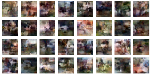
This is super cool. Now we have a deep generative process that can turn random noise into something that looks like our datapoints. It can generate roughly natural-looking images like these:

#### Advantages
In this model a lot of things that are otherwise hard to do are easy to do:
1. generating/imagining data is straightforward
2. inference, i.e. calculating the latent representation from data, is simple
3. you can multiply the distribution with another distribution, making Bayesian calculations for stuff like denoising or superresolution possible.
#### Drawbacks and extensions
I think a drawback of the model is that if you run the diffusion process for too long (i.e. make the model deeper), the mutual information between datapoint and its representation is bound to decrease, due to the stationarity of Brownian motion. I guess this is going to be an important limitation to the depth of these models.
Also, the latent representations at each layer are assumed to be exactly if the same dimensionality and type as the data itsef. So if we are modeling 100x100 images, then all layers in the resulting network will have 100k nodes. I guess this can be overcome by combining variational autoencoders with this method. Also, you can imagine augmenting your space with extra 'pixels' that are only used for richer representations in the intermediate layers.
Anyway, this is super cool, go read the paper.


