[link]
Summary by Alexander Jung 7 years ago
* Stochastic Depth (SD) is a method for residual networks, which randomly removes/deactivates residual blocks during training.
* As such, it is similar to dropout.
* While dropout removes neurons, SD removes blocks (roughly the layers of a residual network).
* One can argue that dropout randomly changes the width of layers, while SD randomly changes the depth of the network.
* One can argue that using dropout is similar to training an ensemble of networks with different layer widths, while using SD is similar to training an ensemble of networks with different depths.
* Using SD has the following advantages:
* It decreases the effects of vanishing gradients, because on average the network is shallower during training (per batch), thereby increasing the gradient that reaches the early blocks.
* It increases training speed, because on average less convolutions have to be applied (due to blocks being removed).
* It has a regularizing effect, because blocks cannot easily co-adapt any more. (Similar to dropout avoiding co-adaption of neurons.)
* If using an increasing removal probability for later blocks: It spends more training time on the early (and thus most important) blocks than on the later blocks.
### How
* Normal formula for a residual block (test and train):
* `output = ReLU(f(input) + identity(input))`
* `f(x)` are usually one or two convolutions.
* Formula with SD (during training):
* `output = ReLU(b * f(input) + identity(input))`
* `b` is either exactly `1` (block survived, i.e. is not removed) or exactly `0` (block was removed).
* `b` is sampled from a bernoulli random variable that has the hyperparameter `p`.
* `p` is the survival probability of a block (i.e. chance to *not* be removed). (Note that this is the opposite of dropout, where higher values lead to more removal.)
* Formula with SD (during test):
* `output = ReLU(p * f(input) + input)`
* `p` is the average probability with which this residual block survives during training, i.e. the hyperparameter for the bernoulli variable.
* The test formula has to be changed, because the network will adapt during training to blocks being missing. Activating them all at the same time can lead to overly strong signals. This is similar to dropout, where weights also have to be changed during test.
* There are two simple schemas to set `p` per layer:
* Uniform schema: Every block gets the same `p` hyperparameter, i.e. the last block has the same chance of survival as the first block.
* Linear decay schema: Survival probability is higher for early layers and decreases towards the end.
* The formula is `p = 1 - (l/L)(1-q)`.
* `l`: Number of the block for which to set `p`.
* `L`: Total number of blocks.
* `q`: Desired survival probability of the last block (0.5 is a good value).
* For linear decay with `q=0.5` and `L` blocks, on average `(3/4)L` blocks will be trained per minibatch.
* For linear decay with `q=0.5` the average speedup will be about `1/4` (25%). If using `q=0.2` the speedup will be ~40%.
### Results
* 152 layer networks with SD outperform identical networks without SD on CIFAR-10, CIFAR-100 and SVHN.
* The improvement in test error is quite significant.
* SD seems to have a regularizing effect. Networks with SD are not overfitting where networks without SD already are.
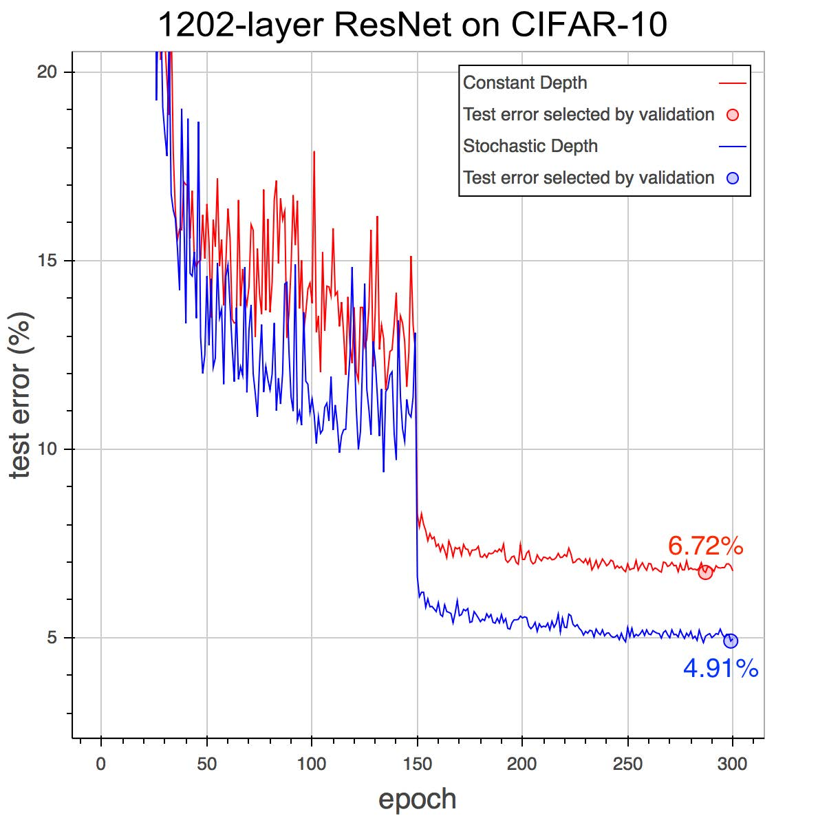
* Even networks with >1000 layers are well trainable with SD.
* The gradients that reach the early blocks of the networks are consistently significantly higher with SD than without SD (i.e. less vanishing gradient).
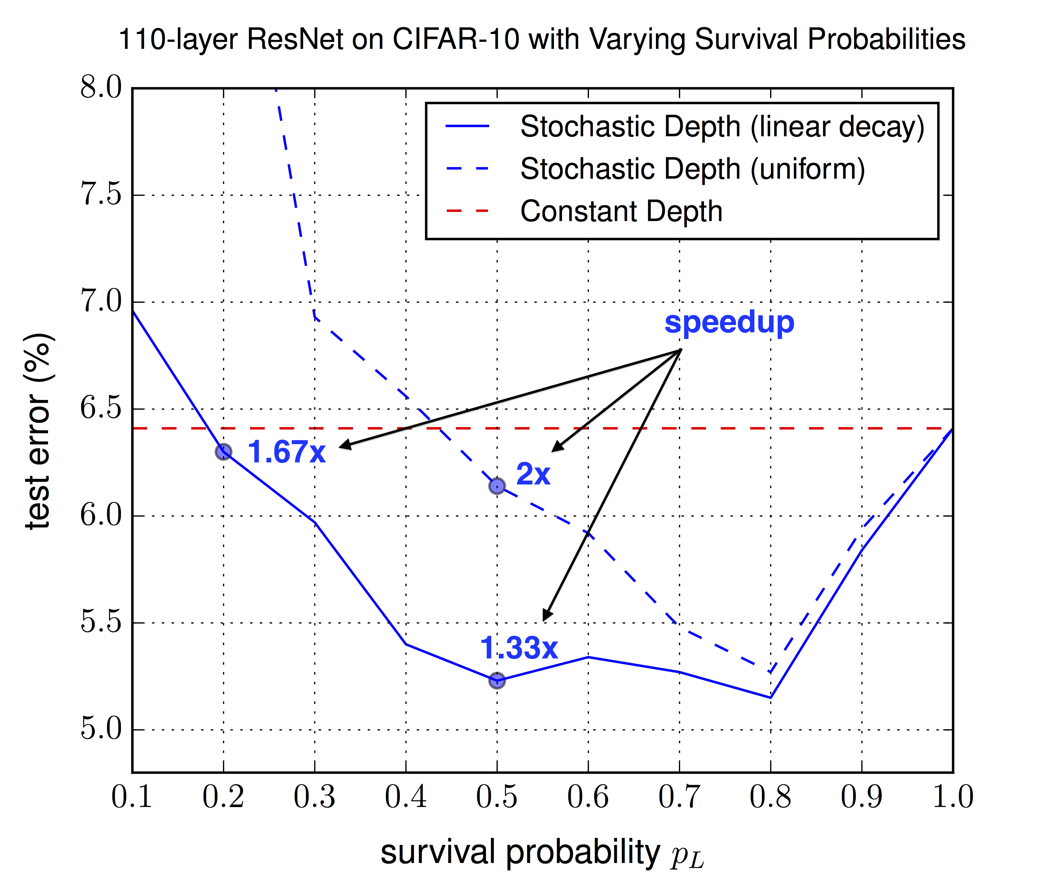
* The linear decay schema consistently outperforms the uniform schema (in test error). The best value seems to be `q=0.5`, though values between 0.4 and 0.8 all seem to be good. For the uniform schema only 0.8 seems to be good.

*Performance on SVHN with 152 layer networks with SD (blue, bottom) and without SD (red, top).*

*Performance on CIFAR-10 with 1202 layer networks with SD (blue, bottom) and without SD (red, top).*

*Optimal choice of the survival probability `p_L` (in this summary `q`) for the last layer, for the uniform schema (same for all other layers) and the linear decay schema (decreasing towards `p_L`). Linear decay performs consistently better and allows for lower `p_L` values, leading to more speedup.*
--------------------
### Rough chapter-wise notes
* (1) Introduction
* Problems of deep networks:
* Vanishing Gradients: During backpropagation, gradients approach zero due to being repeatedly multiplied with small weights. Possible counter-measures: Careful initialization of weights, "hidden layer supervision" (?), batch normalization.
* Diminishing feature reuse: Aequivalent problem to vanishing gradients during forward propagation. Results of early layers are repeatedly multiplied with later layer's (randomly initialized) weights. The total result then becomes meaningless noise and doesn't have a clear/strong gradient to fix it.
* Long training time: The time of each forward-backward increases linearly with layer depth. Current 152-layer networks can take weeks to train on ImageNet.
* I.e.: Shallow networks can be trained effectively and fast, but deep networks would be much more expressive.
* During testing we want deep networks, during training we want shallow networks.
* They randomly "drop out" (i.e. remove) complete layers during training (per minibatch), resulting in shallow networks.
* Result: Lower training time *and* lower test error.
* While dropout randomly removes width from the network, stochastic depth randomly removes depth from the networks.
* While dropout can be thought of as training an ensemble of networks with different depth, stochastic depth can be thought of as training an ensemble of networks with different depth.
* Stochastic depth acts as a regularizer, similar to dropout and batch normalization. It allows deeper networks without overfitting (because 1000 layers clearly wasn't enough!).
* (2) Background
* Some previous methods to train deep networks: Greedy layer-wise training, careful initializations, batch normalization, highway connections, residual connections.
* <Standard explanation of residual networks>
* <Standard explanation of dropout>
* Dropout loses effectiveness when combined with batch normalization. Seems to have basically no benefit any more for deep residual networks with batch normalization.
* (3) Deep Networks with Stochastic Depth
* They randomly skip entire layers during training.
* To do that, they use residual connections. They select random layers and use only the identity function for these layers (instead of the full residual block of identity + convolutions + add).
* ResNet architecture: They use standard residual connections. ReLU activations, 2 convolutional layers (conv->BN->ReLU->conv->BN->add->ReLU). They use <= 64 filters per conv layer.
* While the standard formula for residual connections is `output = ReLU(f(input) + identity(input))`, their formula is `output = ReLU(b * f(input) + identity(input))` with `b` being either 0 (inactive/removed layer) or 1 (active layer), i.e. is a sample of a bernoulli random variable.
* The probabilities of the bernoulli random variables are now hyperparameters, similar to dropout.
* Note that the probability here means the probability of *survival*, i.e. high value = more survivors.
* The probabilities could be set uniformly, e.g. to 0.5 for each variable/layer.
* They can also be set with a linear decay, so that the first layer has a very high probability of survival, while the last layer has a very low probability of survival.
* Linear decay formula: `p = 1 - (l/L)(1-q)` where `l` is the current layer's number, `L` is the total number of layers, `p` is the survival probability of layer `l` and `q` is the desired survival probability of the last layer (e.g. 0.5).
* They argue that linear decay is better, as the early layer extract low level features and are therefor more important.
* The expected number of surviving layers is simply the sum of the probabilities.
* For linear decay with `q=0.5` and `L=54` (i.e. 54 residual blocks = 110 total layers) the expected number of surviving blocks is roughly `(3/4)L = (3/4)54 = 40`, i.e. on average 14 residual blocks will be removed per training batch.
* With linear decay and `q=0.5` the expected speedup of training is about 25%. `q=0.2` leads to about 40% speedup (while in one test still achieving the test error of the same network without stochastic depth).
* Depending on the `q` setting, they observe significantly lower test errors. They argue that stochastic depth has a regularizing effect (training an ensemble of many networks with different depths).
* Similar to dropout, the forward pass rule during testing must be slightly changed, because the network was trained on missing values. The residual formular during test time becomes `output = ReLU(p * f(input) + input)` where `p` is the average probability with which this residual block survives during training.
* (4) Results
* Their model architecture:
* Three chains of 18 residual blocks each, so 3*18 blocks per model.
* Number of filters per conv. layer: 16 (first chain), 32 (second chain), 64 (third chain)
* Between each block they use average pooling. Then they zero-pad the new dimensions (e.g. from 16 to 32 at the end of the first chain).
* CIFAR-10:
* Trained with SGD (momentum=0.9, dampening=0, lr=0.1 after 1st epoch, 0.01 after epoch 250, 0.001 after epoch 375).
* Weight decay/L2 of 1e-4.
* Batch size 128.
* Augmentation: Horizontal flipping, crops (4px offset).
* They achieve 5.23% error (compared to 6.41% in the original paper about residual networks).
* CIFAR-100:
* Same settings as before.
* 24.58% error with stochastic depth, 27.22% without.
* SVHN:
* The use both the hard and easy sub-datasets of images.
* They preprocess to zero-mean, unit-variance.
* Batch size 128.
* Learning rate is 0.1 (start), 0.01 (after epoch 30), 0.001 (after epoch 35).
* 1.75% error with stochastic depth, 2.01% error without.
* Network without stochastic depth starts to overfit towards the end.
* Stochastic depth with linear decay and `q=0.5` gives ~25% speedup.
* 1202-layer CIFAR-10:
* They trained a 1202-layer deep network on CIFAR-10 (previous tests: 152 layers).
* Without stochastic depth: 6.72% test error.
* With stochastic depth: 4.91% test error.
* (5) Analytic experiments
* Vanishing Gradient:
* They analyzed the gradient that reaches the first layer.
* The gradient with stochastic depth is consistently higher (throughout the epochs) than without stochastic depth.
* The difference is very significant after decreasing the learning rate.
* Hyper-parameter sensitivity:
* They evaluated with test error for different choices of the survival probability `q`.
* Linear decay schema: Values between 0.4 and 0.8 perform best. 0.5 is suggested (nearly best value, good spedup). Even 0.2 improves the test error (compared to no stochastic depth).
* Uniform schema: 0.8 performs best, other values mostly significantly worse.
* Linear decay performs consistently better than the uniform schema.


