* The authors define in this paper a special loss function (DeePSiM), mostly for autoencoders.
  * Usually one would use a MSE of euclidean distance as the loss function for an autoencoder. But that loss function basically always leads to blurry reconstructed images.
  * They add two new ingredients to the loss function, which results in significantly sharper looking images.

### How
  * Their loss function has three components:
    * Euclidean distance in image space (i.e. pixel distance between reconstructed image and original image, as usually used in autoencoders)
    * Euclidean distance in feature space. Another pretrained neural net (e.g. VGG, AlexNet, ...) is used to extract features from the original and the reconstructed image. Then the euclidean distance between both vectors is measured.
    * Adversarial loss, as usually used in GANs (generative adversarial networks). The autoencoder is here treated as the GAN-Generator. Then a second network, the GAN-Discriminator is introduced. They are trained in the typical GAN-fashion. The loss component for DeePSiM is the loss of the Discriminator. I.e. when reconstructing an image, the autoencoder would learn to reconstruct it in a way that lets the Discriminator believe that the image is real.
  * Using the loss in feature space alone would not be enough as that tends to lead to overpronounced high frequency components in the image (i.e. too strong edges, corners, other artefacts).
  * To decrease these high frequency components, a "natural image prior" is usually used. Other papers define some function by hand. This paper uses the adversarial loss for that (i.e. learns a good prior).
  * Instead of training a full autoencoder (encoder + decoder) it is also possible to only train a decoder and feed features - e.g. extracted via AlexNet - into the decoder.

### Results
  * Using the DeePSiM loss with a normal autoencoder results in sharp reconstructed images.
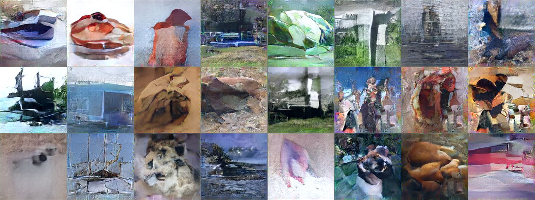
  * Using the DeePSiM loss with a VAE to generate ILSVRC-2012 images results in sharp images, which are locally sound, but globally don't make sense. Simple euclidean distance loss results in blurry images.
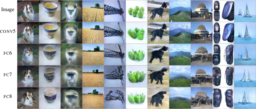
  * Using the DeePSiM loss when feeding only image space features (extracted via AlexNet) into the decoder leads to high quality reconstructions. Features from early layers will lead to more exact reconstructions.
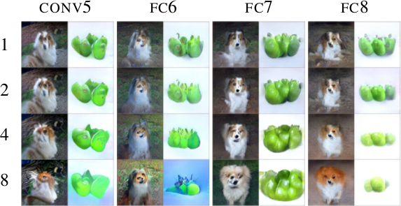
  * One can again feed extracted features into the network, but then take the reconstructed image, extract features of that image and feed them back into the network. When using DeePSiM, even after several iterations of that process the images still remain semantically similar, while their exact appearance changes (e.g. a dog's fur color might change, counts of visible objects change).

![Generated images](https://raw.githubusercontent.com/aleju/papers/master/neural-nets/images/Generating_Images_with_Perceptual_Similarity_Metrics_based_on_Deep_Networks__generated_images.png?raw=true "Generated images")

*Images generated with a VAE using DeePSiM loss.*


![Reconstructed images](https://raw.githubusercontent.com/aleju/papers/master/neural-nets/images/Generating_Images_with_Perceptual_Similarity_Metrics_based_on_Deep_Networks__reconstructed.png?raw=true "Reconstructed images")

*Images reconstructed from features fed into the network. Different AlexNet layers (conv5 - fc8) were used to generate the features. Earlier layers allow more exact reconstruction.*


![Iterated reconstruction](https://raw.githubusercontent.com/aleju/papers/master/neural-nets/images/Generating_Images_with_Perceptual_Similarity_Metrics_based_on_Deep_Networks__reconstructed_multi.png?raw=true "Iterated reconstruction")

*First, images are reconstructed from features (AlexNet, layers conv5 - fc8 as columns). Then, features of the reconstructed images are fed back into the network. That is repeated up to 8 times (rows). Images stay semantically similar, but their appearance changes.*

--------------------

### Rough chapter-wise notes

* (1) Introduction
  * Using a MSE of euclidean distances for image generation (e.g. autoencoders) often results in blurry images.
  * They suggest a better loss function that cares about the existence of features, but not as much about their exact translation, rotation or other local statistics.
  * Their loss function is based on distances in suitable feature spaces.
  * They use ConvNets to generate those feature spaces, as these networks are sensitive towards important changes (e.g. edges) and insensitive towards unimportant changes (e.g. translation).
  * However, naively using the ConvNet features does not yield good results, because the networks tend to project very different images onto the same feature vectors (i.e. they are contractive). That leads to artefacts in the generated images.
  * Instead, they combine the feature based loss with GANs (adversarial loss). The adversarial loss decreases the negative effects of the feature loss ("natural image prior").

* (3) Model
  * A typical choice for the loss function in image generation tasks (e.g. when using an autoencoders) would be squared euclidean/L2 loss or L1 loss.
  * They suggest a new class of losses called "DeePSiM".
  * We have a Generator `G`, a Discriminator `D`, a feature space creator `C` (takes an image, outputs a feature space for that image), one (or more) input images `x` and one (or more) target images `y`. Input and target image can be identical.
  * The total DeePSiM loss is a weighted sum of three components:
    * Feature loss: Squared euclidean distance between the feature spaces of (1) input after fed through G and (2) the target image, i.e. `||C(G(x))-C(y)||^2_2`.
    * Adversarial loss: A discriminator is introduced to estimate the "fakeness" of images generated by the generator. The losses for D and G are the standard GAN losses.
    * Pixel space loss: Classic squared euclidean distance (as commonly used in autoencoders). They found that this loss stabilized their adversarial training.
  * The feature loss alone would create high frequency artefacts in the generated image, which is why a second loss ("natural image prior") is needed. The adversarial loss fulfills that role.
  * Architectures
    * Generator (G):
      * They define different ones based on the task.
      * They all use up-convolutions, which they implement by stacking two layers: (1) a linear upsampling layer, then (2) a normal convolutional layer.
      * They use leaky ReLUs (alpha=0.3).
    * Comparators (C):
      * They use variations of AlexNet and Exemplar-CNN.
      * They extract the features from different layers, depending on the experiment.
    * Discriminator (D):
      * 5 convolutions (with some striding; 7x7 then 5x5, afterwards 3x3), into average pooling, then dropout, then 2x linear, then 2-way softmax.
  * Training details
    * They use Adam with learning rate 0.0002 and normal momentums (0.9 and 0.999).
    * They temporarily stop the discriminator training when it gets too good.
    * Batch size was 64.
    * 500k to 1000k batches per training.

* (4) Experiments
  * Autoencoder
    * Simple autoencoder with an 8x8x8 code layer between encoder and decoder (so actually more values than in the input image?!).
    * Encoder has a few convolutions, decoder a few up-convolutions (linear upsampling + convolution).
    * They train on STL-10 (96x96) and take random 64x64 crops.
    * Using for C AlexNet tends to break small structural details, using Exempler-CNN breaks color details.
    * The autoencoder with their loss tends to produce less blurry images than the common L2 and L1 based losses.
    * Training an SVM on the 8x8x8 hidden layer performs significantly with their loss than L2/L1. That indicates potential for unsupervised learning.
  * Variational Autoencoder
    * They replace part of the standard VAE loss with their DeePSiM loss (keeping the KL divergence term).
    * Everything else is just like in a standard VAE.
    * Samples generated by a VAE with normal loss function look very blurry. Samples generated with their loss function look crisp and have locally sound statistics, but still (globally) don't really make any sense.
  * Inverting AlexNet
    * Assume the following variables:
      * I: An image
      * ConvNet: A convolutional network
      * F: The features extracted by a ConvNet, i.e. ConvNet(I) (feaures in all layers, not just the last one)
    * Then you can invert the representation of a network in two ways:
      * (1) An inversion that takes an F and returns roughly the I that resulted in F (it's *not* key here that ConvNet(reconstructed I) returns the same F again).
      * (2) An inversion that takes an F and projects it to *some* I so that ConvNet(I) returns roughly the same F again.
    * Similar to the autoencoder cases, they define a decoder, but not encoder.
    * They feed into the decoder a feature representation of an image. The features are extracted using AlexNet (they try the features from different layers).
    * The decoder has to reconstruct the original image (i.e. inversion scenario 1). They use their DeePSiM loss during the training.
    * The images can be reonstructed quite well from the last convolutional layer in AlexNet. Chosing the later fully connected layers results in more errors (specifially in the case of the very last layer).
    * They also try their luck with the inversion scenario (2), but didn't succeed (as their loss function does not care about diversity).
    * They iteratively encode and decode the same image multiple times (probably means: image -> features via AlexNet -> decode -> reconstructed image -> features via AlexNet -> decode -> ...). They observe, that the image does not get "destroyed", but rather changes semantically, e.g. three apples might turn to one after several steps.
    * They interpolate between images. The interpolations are smooth.