
|
Welcome to ShortScience.org! |


|
- ShortScience.org is a platform for post-publication discussion aiming to improve accessibility and reproducibility of research ideas.
- The website has 1584 public summaries, mostly in machine learning, written by the community and organized by paper, conference, and year.
- Reading summaries of papers is useful to obtain the perspective and insight of another reader, why they liked or disliked it, and their attempt to demystify complicated sections.
- Also, writing summaries is a good exercise to understand the content of a paper because you are forced to challenge your assumptions when explaining it.
- Finally, you can keep up to date with the flood of research by reading the latest summaries on our Twitter and Facebook pages.
Learning to Segment Object Candidates
Pinheiro, Pedro H. O. and Collobert, Ronan and Dollár, Piotr
arXiv e-Print archive - 2015 via Local Bibsonomy
Keywords: dblp
Pinheiro, Pedro H. O. and Collobert, Ronan and Dollár, Piotr
arXiv e-Print archive - 2015 via Local Bibsonomy
Keywords: dblp


[link]
Facebook has [released a series of papers](https://research.facebook.com/blog/learning-to-segment/) for object segmentation and detection. This paper is the first in that series. This is how modern object detection works (think [RCNN](https://arxiv.org/abs/1311.2524), [Fast RCNN](http://arxiv.org/abs/1504.08083)): 1. A rich set of object proposals (i.e., a set of image regions which are likely to contain an object) is generated using a fast (but possibly imprecise) algorithm. 2. A CNN classifier is applied on each of the proposals. The current paper improves the step 1, i.e., region/object proposals. Most object proposals approaches fall into three categories: * Objectness scoring * Seed Segmentation * Superpixel Merging Current method is different from these three. It share similarities with [Faster R-CNN](https://arxiv.org/abs/1506.01497) in that proposals are generated using a CNN. The method predicts a segmentation mask given an input *patch* and assigns a score corresponding to how likely the patch is to contain an object. ## Model and Training Both mask and score predictions are achieved with a single convolutional network but with multiple outputs. All the convolutional layers except the last few are from VGG-A pretrained model. Each training sample is a triplet of RGB input patch, the binary mask corresponding to the input patch, a label which specifies whether the patch contains an object. A patch is given label 1 only if it satisfies the following constraints: * the patch contains an object roughly centered in the input patch * the object is fully contained in the patch and in a given scale range Note that the network must output a mask for a single object at the center even when multiple objects are present. Figure 1 shows the architecture and sampling for training.  Model is then jointly trained for segmentation and objectness. Negative samples are not used for segmentation. ## Inference During full image inference, model is applied densely at multiple locations and scales. This can be done efficiently since all computations are convolutional like in a fully convolutional network (FCN).  This approach surpasses the previous state of the art by a large margin in both box and segmentation proposal generation.  |

Value Iteration Networks
Tamar, Aviv and Levine, Sergey and Abbeel, Pieter
arXiv e-Print archive - 2016 via Local Bibsonomy
Keywords: dblp
Tamar, Aviv and Levine, Sergey and Abbeel, Pieter
arXiv e-Print archive - 2016 via Local Bibsonomy
Keywords: dblp
|
[link]
Originally posted on my Github repo [paper-notes](https://github.com/karpathy/paper-notes/blob/master/vin.md).
# Value Iteration Networks
By Berkeley group: Aviv Tamar, Yi Wu, Garrett Thomas, Sergey Levine, and Pieter Abbeel
This paper introduces a poliy network architecture for RL tasks that has an embedded differentiable *planning module*, trained end-to-end. It hence falls into a category of fun papers that take explicit algorithms, make them differentiable, embed them in a larger neural net, and train everything end-to-end.
**Observation**: in most RL approaches the policy is a "reactive" controller that internalizes into its weights actions that historically led to high rewards.
**Insight**: To improve the inductive bias of the model, embed a specifically-structured neural net planner into the policy. In particular, the planner runs the value Iteration algorithm, which can be implemented with a ConvNet. So this is kind of like a model-based approach trained with model-free RL, or something. Lol.
NOTE: This is very different from the more standard/obvious approach of learning a separate neural network environment dynamics model (e.g. with regression), fixing it, and then using a planning algorithm over this intermediate representation. This would not be end-to-end because we're not backpropagating the end objective through the full model but rely on auxiliary objectives (e.g. log prob of a state given previous state and action when training a dynamics model), and in practice also does not work well.
NOTE2: A recurrent agent (e.g. with an LSTM policy), or a feedforward agent with a sufficiently deep network trained in a model-free setting has some capacity to learn planning-like computation in its hidden states. However, this is nowhere near as explicit as in this paper, since here we're directly "baking" the planning compute into the architecture. It's exciting.
## Value Iteration
Value Iteration is an algorithm for computing the optimal value function/policy $V^*, \pi^*$ and involves turning the Bellman equation into a recurrence:

This iteration converges to $V^*$ as $n \rightarrow \infty$, which we can use to behave optimally (i.e. the optimal policy takes actions that lead to the most rewarding states, according to $V^*$).
## Grid-world domain
The paper ends up running the model on several domains, but for the sake of an effective example consider the grid-world task where the agent is at some particular position in a 2D grid and has to reach a specific goal state while also avoiding obstacles. Here is an example of the toy task:
The agent gets a reward +1 in the goal state, -1 in obstacles (black), and -0.01 for each step (so that the shortest path to the goal is an optimal solution).
## VIN model
The agent is implemented in a very straight-forward manner as a single neural network trained with TRPO (Policy Gradients with a KL constraint on predictive action distributions over a batch of trajectories). So the only loss function used is to maximize expected reward, as is standard in model-free RL. However, the policy network of the agent has a very specific structure since it (internally) runs value iteration.
First, there's the core Value Iteration **(VI) Module** which runs the recurrence formula (reproducing again):

The input to this recurrence are the two arrays R (the reward array, reward for each state) and P (the dynamics array, the probabilities of transitioning to nearby states with each action), which are of course unknown to the agent, but can be predicted with neural networks as a function of the current state. This is a little funny because the networks take a _particular_ state **s** and are internally (during the forward pass) predicting the rewards and dynamics for all states and actions in the entire environment. Notice, extremely importantly and once again, that at no point are the reward and dynamics functions explicitly regressed to the observed transitions in the environment. They are just arrays of numbers that plug into value iteration recurrence module.
But anyway, once we have **R,P** arrays, in the Grid-world above due to the local connectivity, value iteration can be implemented with a repeated application of convolving **P** over **R**, as these filters effectively *diffuse* the estimated reward function (**R**) through the dynamics model (**P**), followed by max pooling across the actions. If **P** is a not a function of the state, it would simply be the filters in the Conv layer. Notice that posing this as convolution also assumes that the env dynamics are position-invariant. See the diagram below on the right: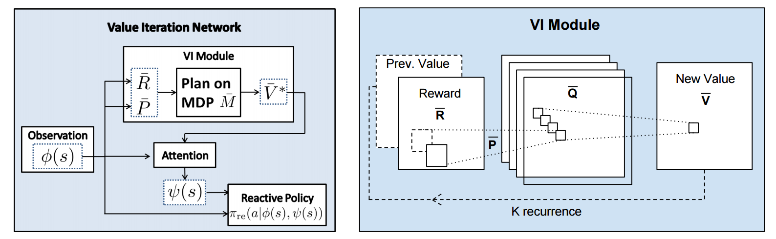
Once the array of numbers that we interpret as holding the estimated $V^*$ is computed after running **K** steps of the recurrence (K is fixed beforehand. For example for a 16x16 map it is 20, since that's a bit more than the amount of steps needed to diffuse rewards across the entire map), we "pluck out" the state-action values $Q(s,.)$ at the state the agent happens to currently be in (by an "attention" operator $\psi$), and (optionally) append these Q values to the feedforward representation of the current state $\phi(s)$, and finally predicting the action distribution.
## Experiments
**Baseline 1**: A vanilla ConvNet policy trained with TRPO. [(50 3x3 filters)\*2, 2x2 max pool, (100 3x3 filters)\*3, 2x2 max pool, FC(100), FC(4), Softmax].
**Baseline 2**: A fully convolutional network (FCN), 3 layers (with a filter that spans the whole image), of 150, 100, 10 filters. i.e. slightly different and perhaps a bit more domain-appropriate ConvNet architecture.
**Curriculum** is used during training where easier environments are trained on first. This is claimed to work better but not quantified in tables. Models are trained with TRPO, RMSProp, implemented in Theano.
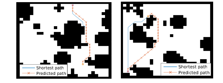
Results when training on **5000** random grid-world instances (hey isn't that quite a bit low?):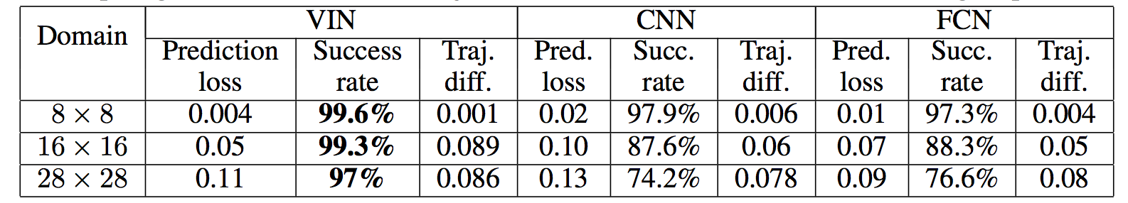
TLDR VIN generalizes better.
The authors also run the model on the **Mars Rover Navigation** dataset (wait what?), a **Continuous Control** 2D path planning dataset, and the **WebNav Challenge**, a language-based search task on a graph (of a subset of Wikipedia). Skipping these because they don't add _too_ much to the core cool idea of the paper.
## Misc
**The good**: I really like this paper because the core idea is cute (the planner is *embedded* in the policy and trained end-to-end), novel (I don't think I saw this idea executed on so far elsewhere), the paper is well-written and clear, and the supplementary materials are thorough.
**On the approach**: Significant challenges remain to make this approach more practicaly viable, but it also seems that much more exciting followup work can be done in this framework. I wish the authors discussed this more in the conclusion. In particular, it seems that one has to explicitly encode the environment connectivity structure in the internal model $\bar{M}$. How much of a problem is this and what could be done about it? Or how could we do the planning in more higher-level abstract spaces instead of the actual low-level state space of the problem? Also, it seems that a potentially nice feature of this approach is that the agent could dynamically "decide" on a reward function at runtime, and the VI module can diffuse it through the dynamics and hence do the planning. A potentially interesting outcome is that the agent could utilize this kind of computation so that an LSTM controller could learn to "emit" reward function subgoals and the VI planner computes how to meet them. A nice/clean division of labor one could hope for in principle.
**The experiments**. Unfortunately, I'm not sure why the authors preferred breadth of experiments and sacrificed depth of experiments. I would have much preferred a more in-depth analysis of the gridworld environment. For instance:
- Only 5,000 training examples are used for training, which seems very little. Presumable, the baselines get stronger as you increase the number of training examples?
- Lack of visualizations: Does the model actually learn the "correct" rewards **R** and dynamics **P**? The authors could inspect these manually and correlate them to the actual model. This would have been reaaaallllyy cool. I also wouldn't expect the model to exactly learn these, but who knows.
- How does the model compare to the baselines in the number of parameters? or FLOPS? It seems that doing VI for 30 steps at each single iteration of the algorithm should be quite expensive.
- The authors should study the performance as a function of the number of recurrences **K**. A particularly funny experiment would be K = 1, where the model would be effectively predicting **V*** directly, without planning. What happens?
- If the output of VI $\psi(s)$ is concatenated to the state parameters, are these Q values actually used? What if all the weights to these numbers are zero in the trained models?
- Why do the authors only evaluate success rate when the training criterion is expected reward?
Overall a very cute idea, well executed as a first step and well explained, with a bit of unsatisfying lack of depth in the experiments in favor of breadth that doesn't add all that much.
2 Comments
  |

Deep Residual Learning for Image Recognition
He, Kaiming and Zhang, Xiangyu and Ren, Shaoqing and Sun, Jian
arXiv e-Print archive - 2015 via Local Bibsonomy
Keywords: dblp
He, Kaiming and Zhang, Xiangyu and Ren, Shaoqing and Sun, Jian
arXiv e-Print archive - 2015 via Local Bibsonomy
Keywords: dblp
|
[link]
Deeper networks should never have a higher **training** error than smaller ones. In the worst case, the layers should "simply" learn identities. It seems as this is not so easy with conventional networks, as they get much worse with more layers. So the idea is to add identity functions which skip some layers. The network only has to learn the **residuals**.

Advantages:

* Learning the identity becomes learning 0 which is simpler
* Loss in information flow in the forward pass is not a problem anymore
    * No vanishing / exploding gradient
* Identities don't have parameters to be learned

## Evaluation

The learning rate starts at 0.1 and is divided by 10 when the error plateaus. Weight decay of 0.0001 ($10^{-4}$), momentum of 0.9. They use mini-batches of size 128.

* ImageNet ILSVRC 2015: 3.57% (ensemble)
* CIFAR-10: 6.43%
* MS COCO: 59.0% mAp@0.5 (ensemble)
* PASCAL VOC 2007: 85.6% mAp@0.5
* PASCAL VOC 2012: 83.8% mAp@0.5

## See also

* [DenseNets](http://www.shortscience.org/paper?bibtexKey=journals/corr/1608.06993)
|

Using Fast Weights to Attend to the Recent Past
Jimmy Ba and Geoffrey Hinton and Volodymyr Mnih and Joel Z. Leibo and Catalin Ionescu
arXiv e-Print archive - 2016 via Local arXiv
Keywords: stat.ML, cs.LG, cs.NE
First published: 2016/10/20 (7 years ago)
Abstract: Until recently, research on artificial neural networks was largely restricted to systems with only two types of variable: Neural activities that represent the current or recent input and weights that learn to capture regularities among inputs, outputs and payoffs. There is no good reason for this restriction. Synapses have dynamics at many different time-scales and this suggests that artificial neural networks might benefit from variables that change slower than activities but much faster than the standard weights. These "fast weights" can be used to store temporary memories of the recent past and they provide a neurally plausible way of implementing the type of attention to the past that has recently proved very helpful in sequence-to-sequence models. By using fast weights we can avoid the need to store copies of neural activity patterns.
more
less
Jimmy Ba and Geoffrey Hinton and Volodymyr Mnih and Joel Z. Leibo and Catalin Ionescu
arXiv e-Print archive - 2016 via Local arXiv
Keywords: stat.ML, cs.LG, cs.NE
First published: 2016/10/20 (7 years ago)
Abstract: Until recently, research on artificial neural networks was largely restricted to systems with only two types of variable: Neural activities that represent the current or recent input and weights that learn to capture regularities among inputs, outputs and payoffs. There is no good reason for this restriction. Synapses have dynamics at many different time-scales and this suggests that artificial neural networks might benefit from variables that change slower than activities but much faster than the standard weights. These "fast weights" can be used to store temporary memories of the recent past and they provide a neurally plausible way of implementing the type of attention to the past that has recently proved very helpful in sequence-to-sequence models. By using fast weights we can avoid the need to store copies of neural activity patterns.
|
[link]
This paper presents a recurrent neural network architecture in which some of the recurrent weights dynamically change during the forward pass, using a hebbian-like rule. They correspond to the matrices $A(t)$ in the figure below:

These weights $A(t)$ are referred to as *fast weights*. Comparatively, the recurrent weights $W$ are referred to as slow weights, since they are only changing due to normal training and are otherwise kept constant at test time.
More specifically, the proposed fast weights RNN compute a series of hidden states $h(t)$ over time steps $t$, but, unlike regular RNNs, the transition from $h(t)$ to $h(t+1)$ consists of multiple ($S$) recurrent layers $h_1(t+1), \dots, h_{S-1}(t+1), h_S(t+1)$, defined as follows:
$$h_{s+1}(t+1) = f(W h(t) + C x(t) + A(t) h_s(t+1))$$
where $f$ is an element-wise non-linearity such as the ReLU activation. The next hidden state $h(t+1)$ is simply defined as the last "inner loop" hidden state $h_S(t+1)$, before moving to the next time step.
As for the fast weights $A(t)$, they too change between time steps, using the hebbian-like rule:
$$A(t+1) = \lambda A(t) + \eta h(t) h(t)^T$$
where $\lambda$ acts as a decay rate (to partially forget some of what's in the past) and $\eta$ as the fast weight's "learning rate" (not to be confused with the learning rate used during backprop). Thus, the role played by the fast weights is to rapidly adjust to the recent hidden states and remember the recent past.
In fact, the authors show an explicit relation between these fast weights and memory-augmented architectures that have recently been popular. Indeed, by recursively applying and expending the equation for the fast weights, one obtains
$$A(t) = \eta \sum_{\tau = 1}^{\tau = t-1}\lambda^{t-\tau-1} h(\tau) h(\tau)^T$$
*(note the difference with Equation 3 of the paper... I think there was a typo)* which implies that when computing the $A(t) h_s(t+1)$ term in the expression to go from $h_s(t+1)$ to $h_{s+1}(t+1)$, this term actually corresponds to
$$A(t) h_s(t+1) = \eta \sum_{\tau =1}^{\tau = t-1} \lambda^{t-\tau-1} h(\tau) (h(\tau)^T h_s(t+1))$$
i.e. $A(t) h_s(t+1)$ is a weighted sum of all previous hidden states $h(\tau)$, with each hidden states weighted by an "attention weight" $h(\tau)^T h_s(t+1)$. The difference with many recent memory-augmented architectures is thus that the attention weights aren't computed using a softmax non-linearity.
Experimentally, they find it beneficial to use [layer normalization](https://arxiv.org/abs/1607.06450). Good values for $\eta$ and $\lambda$ seem to be 0.5 and 0.9 respectively. I'm not 100% sure, but I also understand that using $S=1$, i.e. using the fast weights only once per time steps, was usually found to be optimal. Also see Figure 3 for the architecture used on the image classification datasets, which is slightly more involved.
The authors present a series 4 experiments, comparing with regular RNNs (IRNNs, which are RNNs with ReLU units and whose recurrent weights are initialized to a scaled identity matrix) and LSTMs (as well as an associative LSTM for a synthetic associative retrieval task and ConvNets for the two image datasets). Generally, experiments illustrate that the fast weights RNN tends to train faster (in number of updates) and better than the other recurrent architectures. Surprisingly, the fast weights RNN can even be competitive with a ConvNet on the two image classification benchmarks, where the RNN traverses glimpses from the image using a fixed policy.
**My two cents**
This is a very thought provoking paper which, based on the comparison with LSTMs, suggests that fast weights RNNs might be a very good alternative. I'd be quite curious to see what would happen if one was to replace LSTMs with them in the myriad of papers using LSTMs (e.g. all the Seq2Seq work). Intuitively, LSTMs seem to be able to do more than just attending to the recent past. But, for a given task, if one was to observe that fast weights RNNs are competitive to LSTMs, it would suggests that the LSTM isn't doing something that much more complex. So it would be interesting to determine what are the tasks where the extra capacity of an LSTM is actually valuable and exploitable. Hopefully the authors will release some code, to facilitate this exploration.
The discussion at the end of Section 3 on how exploiting the "memory augmented" view of fast weights is useful to allow the use of minibatches is interesting. However, it also suggests that computations in the fast weights RNN scales quadratically with the sequence size (since in this view, the RNN technically must attend to all previous hidden states, since the beginning of the sequence). This is something to keep in mind, if one was to consider applying this to very long sequences (i.e. much longer than the hidden state dimensionality).
Also, I don't quite get the argument that the "memory augmented" view of fast weights is more amenable to mini-batch training. I understand that having an explicit weight matrix $A(t)$ for each minibatch sequence complicates things. However, in the memory augmented view, we also have a "memory matrix" that is different for each sequence, and yet we can handle that fine. The problem I can imagine is that storing a *sequence of arbitrary weight matrices* for each sequence might be storage demanding (and thus perhaps make it impossible to store a forward/backward pass for more than one sequence at a time), while the implicit memory matrix only requires appending a new row at each time step. Perhaps the argument to be made here is more that there's already mini-batch compatible code out there for dealing with the use of a memory matrix of stored previous memory states.
This work strikes some (partial) resemblance to other recent work, which may serve as food for thought here. The use of possibly multiple computation layers between time steps reminds me of [Adaptive Computation Time (ACT) RNN]( http://www.shortscience.org/paper?bibtexKey=journals/corr/Graves16). Also, expressing a backpropable architecture that involves updates to weights (here, hebbian-like updates) reminds me of recent work that does backprop through the updates of a gradient descent procedure (for instance as in [this work]( http://www.shortscience.org/paper?bibtexKey=conf/icml/MaclaurinDA15)).
Finally, while I was familiar with the notion of fast weights from the work on [Using Fast Weights to Improve Persistent Contrastive Divergence](http://people.ee.duke.edu/~lcarin/FastGibbsMixing.pdf), I didn't realize that this concept dated as far back as the late 80s. So, for young researchers out there looking for inspiration for research ideas, this paper confirms that looking at the older neural network literature for inspiration is probably a very good strategy :-)
To sum up, this is really nice work, and I'm looking forward to the NIPS 2016 oral presentation of it!
|

Inception-v4, Inception-ResNet and the Impact of Residual Connections on Learning
Szegedy, Christian and Ioffe, Sergey and Vanhoucke, Vincent
arXiv e-Print archive - 2016 via Local Bibsonomy
Keywords: dblp
Szegedy, Christian and Ioffe, Sergey and Vanhoucke, Vincent
arXiv e-Print archive - 2016 via Local Bibsonomy
Keywords: dblp
|
[link]
This paper presents a combination of the inception architecture with residual networks. This is done by adding a shortcut connection to each inception module. This can alternatively be seen as a resnet where the 2 conv layers are replaced by a (slightly modified) inception module. The paper (claims to) provide results against the hypothesis that adding residual connections improves training, rather increasing the model size is what makes the difference. |
