
|
Welcome to ShortScience.org! |


|
- ShortScience.org is a platform for post-publication discussion aiming to improve accessibility and reproducibility of research ideas.
- The website has 1584 public summaries, mostly in machine learning, written by the community and organized by paper, conference, and year.
- Reading summaries of papers is useful to obtain the perspective and insight of another reader, why they liked or disliked it, and their attempt to demystify complicated sections.
- Also, writing summaries is a good exercise to understand the content of a paper because you are forced to challenge your assumptions when explaining it.
- Finally, you can keep up to date with the flood of research by reading the latest summaries on our Twitter and Facebook pages.
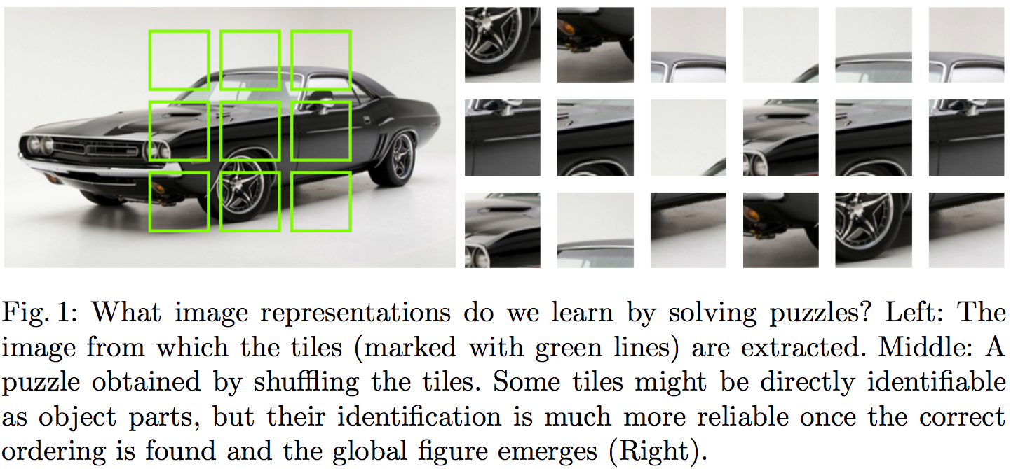
Unsupervised Learning of Visual Representations by Solving Jigsaw Puzzles
Noroozi, Mehdi and Favaro, Paolo
arXiv e-Print archive - 2016 via Local Bibsonomy
Keywords: dblp
Noroozi, Mehdi and Favaro, Paolo
arXiv e-Print archive - 2016 via Local Bibsonomy
Keywords: dblp


[link]
The core idea behind this paper is powerfully simple. The goal is to learn useful representations from unlabelled data, useful in the sense of helping supervised object classification. This paper does this by chopping up images into a set of little jigsaw puzzle, scrambling the pieces, and asking a deep neural network to learn to reassemble them in the correct constellation. A picture is worth a thousand words, so here is Figure 1 taken from the paper explaining this visually:
#### Summary of this note:
- I note the similarities to denoising autoencoders, which motivate my question: "Can this method equivalently represent the data generating distribution?"
- I consider a toy example with just two jigsaw pieces, and consider using an objective like this to fit a generative model $Q$ to data
- I show how the jigsaw puzzle training procedure corresponds to minimising a difference of KL divergences
- Conclude that the algorithm ignores some aspects of the data generating distribution, and argue that in this case it can be a good thing
#### What does this learn do?
This idea seems to make a lot of sense. But to me, one interesting question is the following:
`What does a network trained to solve jigsaw puzzle learn about the data generating distribution?`
#### Motivating example: denoising autoencoders
At one level, this jigsaw puzzle approach bears similarities to denoising autoencoders (DAEs): both methods are self-supervised: they take an unlabelled data and generate a synthetic supervised learning task. You can also interpret solving jigsaw puzzles as a special case 'undoing corruption' thus fitting a more general definition of autoencoders (Bengio et al, 2014).
DAEs have been shown to be related to score matching (Vincent, 2000), and that they learn to represent gradients of the log-probability-density-function of the data generating distribution (Alain et al, 2012). In this sense, autoencoders equivalently represent a complete probability distribution up to normalisation. This concept is also exploited in Harri Valpola's work on ladder networks (Rasmus et al, 2015)
So I was curious if I can find a similar neat interpretation of what really is going on in this jigsaw puzzle thing. If you equivalently represent all aspects of a probability distribution this way? Are there aspects that this representation ignores? Would it correspond to a consistent denisty estimation/generative modelling method in any sense? Below is my attempt to figure this out.
#### A toy case with just two jigsaw pieces
To simplify things, let's just consider a simpler jigsaw puzzle problem with just two jigsaw positions instead of 9, and in such a way that there are no gaps between puzzle pieces, so image patches (now on referred to as data $x$) can be partitioned exactly into pieces.
Let's assume our datapoints $x^{(n)}$ are drawn i.i.d. from an unknown distribution $P$, and that $x$ can be partitioned into two chunks $x_1$ and $x_2$ of equivalent dimensionality, such that $x=(x_1,x_2)$ by definition. Let's also define the permuted/scrambled version of a datapoint $x$ as $\hat{x}:=(x_2,x_1)$.
The jigsaw puzzle problem can be formulated in the following way: we draw a datapoint $x$ from $P$. We also independently draw a binary 'label' $y$ from a Bernoulli($\frac{1}{2}$) distribution, i.e. toss a coin. If $y=1$ we set $z=x$ otherwise $z=\hat{x}$.
Our task is to build a predictior, $f$, which receives as input $z$ and infers the value of $y$ (outputs the probability that its value is $1$). In other words, $f$ tries to guess the correct ordering of the chunks that make up the randomly scrambled datapoint $z$, thereby solving the jigsaw puzzle. The accuracy of the predictor is evaluated using the log-loss, a.k.a. binary cross-entropy, as it is common in binary classification problems:
$$ \mathcal{L}(f) = - \frac{1}{2} \mathbb{E}_{x\sim P} \left[\log f(x) + \log (1 - f(\hat{x}))\right] $$
Let's consider the case when we express the predictor $f$ in terms of a generative model $Q$ of $x$. $Q$ is an approximation to $P$, and has some parameters $\theta$ which we can tweak. For a given $\theta$, the posterior predictive distribution of $y$ takes the following form:
$$ f(z,\theta) := Q(y=1\vert z;\theta) = \frac{Q(z;\theta)}{Q(z;\theta) + Q(\hat{z};\theta)},
$$
where $\hat{z}$ denotes the scrambled/permuted version of $z$. Notice that when $f$ is defined this way the following property holds:
$$ 1 - f(\hat{x};\theta) = f(x;\theta),
$$
so we can simplify the expression for the log-loss to finally obtain:
\begin{align} \mathcal{L}(\theta) &= - \mathbb{E}_{x \sim P} \log Q(x;\theta) + \mathbb{E}_{x \sim P} \log [Q(x;\theta) + Q(\hat{x};\theta)]\\ &= \operatorname{KL}[P\|Q_{\theta}] - \operatorname{KL}\left[P\middle\|\frac{Q_{\theta}(x)+Q_{\theta}(\hat{x})}{2}\right] + \log(2) \end{align}
So we already see that using the jigsaw objective to train a generative model reduces to minimising the difference between two KL divergences. It's also possible to reformulate the loss as:
$$ \mathcal{L}(\theta) = \operatorname{KL}[P\|Q_{\theta}] - \operatorname{KL}\left[\frac{P(x) + P(\hat{x})}{2}\middle\|\frac{Q_{\theta}(x)+Q_{\theta}(\hat{x})}{2}\right] - \operatorname{KL}\left[P\middle\|\frac{P(x) + P(\hat{x})}{2}\right] + \log(2) $$
Let's look at what the different terms do:
- The first term is the usual KL divergence that would correspond to maximum likelihood. So it just tries to make $Q$ as close to $P$ as possible.
- The second term is a bit weird, particularly as comes into the formula with a negative sign. The KL divergence is $0$ if $Q$ and $P$ define the distribution over the set of jigsaw pieces ${x_1,x_2}$. Notice, I used set notation here, so the ordering does not matter. In a way this term tells the loss function: don't bother modelling what the jigsaw pieces are, only model how they fit together.
- The last terms are constant wrt. $\theta$ so we don't need to worry about them.
#### Not a proper scoring rule (and it's okay)
From the formula above it is clear that the jigsaw training objective wouldn't be a proper scoring rule, as it is not uniquely minimised by $Q=P$ in all cases. Here are two counterexamples where the objective fails to capture all aspects of $P$:
Consider the case when $P=\frac{P(x) + P(\hat{x})}{2}$, that is, when $P$ is completely insensitive to the ordering of jigsaw pieces. As long as $Q$ also has this property $Q = \frac{Q(x) + Q(\hat{x})}{2}$, all KL divergences are $0$ and the jigsaw objective is constant with respect $\theta$. Indeed, it is impossible in this case for any classifier to surpass chance level in the jigsaw problem.
Another simple example to consider is a two-dimensional binary $P$. Here, the jigsaw objective only cares about the value of $Q(0,1)$ relative to $Q(1,0)$, but completely insensitive to $Q(1,1)$ and $Q(0,0)$. In other words, we don't really care how often $0$s and $1$s appear, we just want to know which one is likelier to be on the left or the right side.
This is all fine because we don't use this technique for generative modelling. We want to use it for representation learning, so it's okay to ignore some aspects of $P$.
#### Representation learning
I think this method seems like a really promising direction for unsupervised representation learning. In my mind representation learning needs either:
- strong prior assumptions about what variables/aspects of data are behaviourally relevant, or relevant to the tasks we want to solve with the representations.
- at least a little data in a semi-supervised setting to inform us about what is relevant and what is not.
Denoising autoencoders (with L2 reconstruction loss) and maximum likelihood training try to represent all aspects of the data generating distribution, down to pixel level. We can encode further priors in these models in various ways, either by constraining the network architecture or via probabilistic priors over latent variables.
The jigsaw method encodes prior assumptions into the training procedure: that the structure of the world (relative position of parts) is more important to get right than the low-level appearance of parts. This is probably a fair assumption.
 |

A Maximum Entropy Approach to Natural Language Processing
Berger, Adam L. and Pietra, Stephen Della and Pietra, Vincent J. Della
Computational Linguistics - 1996 via Local Bibsonomy
Keywords: dblp
Berger, Adam L. and Pietra, Stephen Della and Pietra, Vincent J. Della
Computational Linguistics - 1996 via Local Bibsonomy
Keywords: dblp
|
[link]
A fundamental paper by Adam Berger and his colleagues at IBM Watson Research Center presents a thorough guide on how to apply maximum entropy (ME) modelling in NLP. Authors follow the principle of maximum entropy and show the optimality of their procedure as well as its duality relationship with the maximum log-likelihood estimation. Importantly, the paper proposes a method for automatic feature selection, perhaps the most critical step in the entire approach. Empirical results from Candide, an IBM’s automatic machine-translation system, demonstrate the capabilities of ME models. Both originality and wide range of possible applications made the paper to stand out and led to the deserved accolades. Many practical NLP problems impose constraints in terms of data or explicit statements, while requiring minimal assumption on the underlying distributions. Laplace advocated that in this scenario the best strategy is to treat everything as equal as possible, while being consistent with the observed facts. Authors follow Laplace’s philosophy and propose to use entropy as a measure of uniformly distributed uncertainty. They employ the principle of maximum entropy to choose the best performing model, which simply states that the optimal model is the one that has the largest entropy. For a given set of features f they model its expected value using the empirical data distribution p(x,y) as p(f) = sum[p(x,y)*f(x,y)] = sum[p(y|x)*p(x)*f(x,y)]. By replacing the conditional probability p(y|x) with its entropy, they obtain the objective function H(p) = -sum[p(x)*p(y|x)*log(p(y|x))]. The optimal distribution p* is then defined as p* = argmax(H(p)). Note that this optimization usually requires a numerical solution. Therefore, authors employ Lagrange multipliers L(p, lambda) = H(p) + sum[lambda_i * (p(f_i) – p_tilda(f_i))], which yields p_lambda(y|x) = 1/Z * exp(sum[lambda_i * f_i(x,y)]) and L(lambda) = -sum[p(x)*log(Z)] + sum[lambda_i*p(f_i)], where Z is a normalizing constant. The unconstraint dual problem then becomes lambda = argmax(L(lambda)). Interestingly, that L is exactly equal to the log-likelihood of the data sample, which implies that MLE and ME are dual and ensures the optimality of ME, since it converges to the best fit of the data. To estimate the model parameters, authors proposed an iterative scaling method, which update lambda by solving sum[p(x)*p(y|x)*f_i(x,y)*exp(delta_lambda * f(x,y))] = p(f_i). The choice of features f is apparently the most critical step in the procedure. Authors propose a simple approach of feature selection by iteratively adding a feature f_new that maximizes the increase in entropy. They continue expanding the set of features until the cross-validation results converge. To evaluate ME approach, the authors applied it to context-sensitive word-translation, sentence segmentation, and word reordering problems. These applications demonstrate the efficacy of ME techniques for performing context-sensitive modelling and the paper undoubtedly deserves the attention it gained. For example, in word reordering the model outperform a simple baseline model by 10%. However, a deeper analysis of the feature selection could benefit it. The proposed feature selection method is computationally expensive, as it iteratively calls optimization subroutine and involves a cross-validation step. Moreover, authors skip the discussion on overfitting and the choice of the initial pool of the features. They imply that the features have to be designed manually, which makes the approach impractical for large diverse problems. Therefore, further developments in dimensionality reduction and feature extraction could benefit ME. |

Development and validation of a continuous measure of patient condition using the Electronic Medical Record
Rothman, Michael J. and Rothman, Steven I. and IV, Joseph Beals
Journal of Biomedical Informatics - 2013 via Local Bibsonomy
Keywords: dblp
Rothman, Michael J. and Rothman, Steven I. and IV, Joseph Beals
Journal of Biomedical Informatics - 2013 via Local Bibsonomy
Keywords: dblp
|
[link]
#### Goal: + Development and validation of a continuous score for patient assessment (to be used both outside and inside intensive care). + Prior work: Modified Early Warning Score (MEWS) identifies 44% of intensive care transfers occurring within the next 12 hours. Generates 69 false positives for each correctly identified event. #### Dataset: Model Creation | Model Validation ---------------|------------------ 22,265 patients admitted to the *Sarasota Memorial Hospital* (SMH) between Jan/2004 and Dec/2004 | 32341 patients admitted to the SMH between Sep/2007 and Jun/2009 | 45,771 patients admitted to the SMH between Jan/2008 and May/2010 | 32,416 patients admitted to *Abigton Memorial Hospital* (AMH) between Jul/2009 and Jun/2010 | 19,402 patients admitted between Jul/2008 and Nov/2008 in *Hospital C*. + ~ 7000 variables, 500 laboratory tests. + Constraints: + Variables should be related to the patient's condition + Collected with some frequency + Susceptible to variation during patient stay in the hospital + Focus: "How the patient is" not "Who the patient is" + The constraints reduce the number of candidate variables to 43 (13 nurse assessments, 6 vital signs and 23 laboratory tests) #### Rothman Index: + The Rothman Index is based on the "Excess Risk" associated with each of the variables: + The excess risk is determined by the increase (in percentage points) of the mortality at 1 year identified for that variable. In the best case, the "excess" risk is zero and the Rothman Index equals 100. 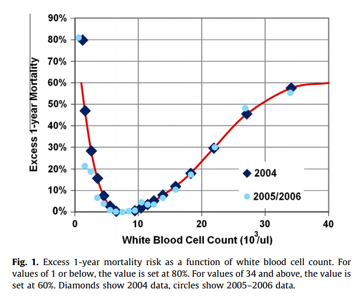 + The excess risk somewhat resembles the *impact coding* for categorical variables. One must always be careful that there is no data snooping. + The index consists of the 26 variables below. They were chosen from the 43 candidates using a *forward stepwise logistic regression* with the patients of the model creation dataset (criterion p-value <0.05). Note that the logistic regression is used only to choose the variables. The Rothman Index is not a regression model itself. 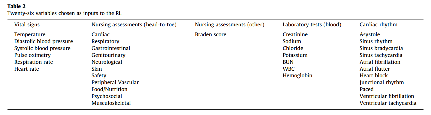 + The lab tests are collected less frequently. The score is divided into two parts (one that takes into account the laboratory variables and another that does not take into account). 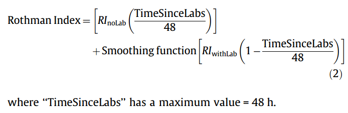 + *TimeSinceLabs* has a maximum value of 48 hours. #### Results: + Outcomes: + Mortality in 24h + Unplanned readmission in 30 days + Discharge + Rothman Index is correlated with discharge category (Home, Home healthcare, Rehab, Skilled Nursing Facility, Hospice, Death) |Mortality in 24h || Readmission in 30 days || Discriminates type of discharge| | |-------------|-|-----------------------|-|------------------------|-------------------------------| | Hospital| AUC | Hospital | AUC | Hospital | AUC| |SMH | 0.933 (0.915-0.930) | SMH | 0.62 (0.61-0.63) | SMH | 0.923 (0.915-0.930)| |AMH | 0.948 (0.960-0.970) | AMH | *| AMH | 0.965 (0.960-0.970)| |C | 0.929 (0.919-0.940) | C | *| C| 0.915 (0.900-0.931) | (*) in the case of readmission in 30 days it was possible to only identify the patients of the SMH hospital. + Tracking the Rothman Index and correlating it with events during hospital stay: 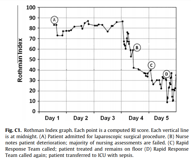 #### Discussion: + Choice of 1-year mortality to calculate excess risk: + Instead of in-hospital death, which is relatively rare (approximately 1—2% of patients), the model is based on 1-year post discharge mortality, where death is far more common (approximately 10% of patients). + Improve the *signal strength* to determine the relationships between clinical measures and risk. + Outcome should be sufficiently frequent and a plausible surrogate for the patient condition. In this case, the risk tries to quantify *distance from death*. + The Rothman index is not designed to predict any specific outcome. + Caveat: Results should have included precision/recall analysis. For risk assessment it is important to evaluate the rate of false alarms per one true positive. |

Decibel: The Relational Dataset Branching System
Maddox, Michael and Goehring, David and Elmore, Aaron J. and Madden, Samuel and Parameswaran, Aditya G. and Deshpande, Amol
Proceedings of the VLDB Endowment (PVLDB) - 2016 via Local Bibsonomy
Keywords: dblp
Maddox, Michael and Goehring, David and Elmore, Aaron J. and Madden, Samuel and Parameswaran, Aditya G. and Deshpande, Amol
Proceedings of the VLDB Endowment (PVLDB) - 2016 via Local Bibsonomy
Keywords: dblp
|
[link]
Decibel is like git for relational data. Often, teams need to simultaneously query, analyze, clean, or curate a collection of data without clobbering each other's work. Currently, the best solution available involves each team member making copies of the entire database. This is undesirable for a number of reasons: - Data is stored very redundantly, wasting a huge amount of storage. - It is difficult to share or merge changes made to local snapshots of the data. - There is no systematic way to say which version of the data was used for a given experiment. Version control solves these problems, but existing version control systems (e.g. git) have a couple of shortcomings when applied naively to large datasets: - Using distributed version control systems like git, clients clone an entire copy of a repository's contents. This is infeasible when working with large datasets. - Version control systems like git operate on arbitrary data and do not understand the structure of relational data. This makes certain operations like generic diffing a bad fit. - Systems like git do not support high-level data management or query APIs. Decibel manages datasets which are collections of relations, and each relation's schema includes an immutable primary key which is used to track the version of each row. Beginning with an initial snapshot of a dataset, users can check out, branch, and commit changes to the data set in a style very similar to git. When data is merged, non-conflicting changes to separate columns of the same row are both applied. If conflicting changes to the same column of the same row occur, one branch's changes take priority. Diffing two tables across two branches results in a table of insertions and deletions. Finally, data can be queried across versions using VQuel: a query language which is notably not SQL. This paper describes three physical realizations of Decibel's logical data model. 1. In a tuple-first representation, tables contain every version of every row, and each row is annotated with a bitmap indicating the set of versions in which the row is live. In a tuple-oriented approach, each of N tuples comes with a B-bit bitmap for B branches. In a branch-oriented approach, there are B N-bit bitmaps. 2. In a version-first representation, all the changes made to a table in a branch are stored together in the same file, and these branched files contain pointers to their ancestors forming a directed acyclic graph. 3. In a hybrid representation, data is stored similarly to the version-first approach, but each of the branched files (called segments) includes a segment index: a bitmap, like in the tuple-first representation, that tracks the liveness of each row for all descendent branches. Moreover, there is a single branch-segment bitmap which for each branch, records the set of segments with a tuple live in that branch. The tuple-first representation is good for multi-version queries, the version-first representation is good for single-version queries, and the hybrid approach is good at both. This paper also presents a versioned database benchmarking framework in the form of a set of branching strategies and characteristic queries to analyze Decibel and any future versioned databases. Commentary. A git-like versioned relational database seems like a great idea! This paper focuses on how to implement and analyze such a database efficiently; it focuses less on the higher-level semantics of data versioning. Notably, two unanswered questions stuck out to me that seem like interesting areas for future research. 1. The current merging strategy seems inconvenient, if not inconsistent. Imagine a table R(key, a, b) with the invariant that a + b < 10. Imagine branch b1 updates a tuple (0, 0, 0) to (0, 9, 0) and branch b2 updates it to (0, 0, 9). If these tuples are merged, the tuple becomes (0, 9, 9) violating the invariant. In systems like git, users can manually inspect and verify the correctness of the merge, but if a large dataset is being merged, this becomes infeasible. I think more research is needed to determine if this strategy is good enough and won't cause problems in practice. Or if it is insufficient, what merging strategies can be applied on large datasets. Perhaps ideas could be borrowed from CRDT literature; if all columns were semilattices, the columns could be merged in a sane way. 2. How useful is diffing when dealing with large datasets? When working with git, even a modestly sized diff can become confusing. Would a non-trivial diff of a large dataset be incomprehensible? |

An Actor-Critic Algorithm for Sequence Prediction
Dzmitry Bahdanau and Philemon Brakel and Kelvin Xu and Anirudh Goyal and Ryan Lowe and Joelle Pineau and Aaron Courville and Yoshua Bengio
arXiv e-Print archive - 2016 via Local arXiv
Keywords: cs.LG
First published: 2016/07/24 (9 years ago)
Abstract: We present an approach to training neural networks to generate sequences using actor-critic methods from reinforcement learning (RL). Current log-likelihood training methods are limited by the discrepancy between their training and testing modes, as models must generate tokens conditioned on their previous guesses rather than the ground-truth tokens. We address this problem by introducing a \textit{critic} network that is trained to predict the value of an output token, given the policy of an \textit{actor} network. This results in a training procedure that is much closer to the test phase, and allows us to directly optimize for a task-specific score such as BLEU. Crucially, since we leverage these techniques in the supervised learning setting rather than the traditional RL setting, we condition the critic network on the ground-truth output. We show that our method leads to improved performance on both a synthetic task, and for German-English machine translation. Our analysis paves the way for such methods to be applied in natural language generation tasks, such as machine translation, caption generation, and dialogue modelling.
more
less
Dzmitry Bahdanau and Philemon Brakel and Kelvin Xu and Anirudh Goyal and Ryan Lowe and Joelle Pineau and Aaron Courville and Yoshua Bengio
arXiv e-Print archive - 2016 via Local arXiv
Keywords: cs.LG
First published: 2016/07/24 (9 years ago)
Abstract: We present an approach to training neural networks to generate sequences using actor-critic methods from reinforcement learning (RL). Current log-likelihood training methods are limited by the discrepancy between their training and testing modes, as models must generate tokens conditioned on their previous guesses rather than the ground-truth tokens. We address this problem by introducing a \textit{critic} network that is trained to predict the value of an output token, given the policy of an \textit{actor} network. This results in a training procedure that is much closer to the test phase, and allows us to directly optimize for a task-specific score such as BLEU. Crucially, since we leverage these techniques in the supervised learning setting rather than the traditional RL setting, we condition the critic network on the ground-truth output. We show that our method leads to improved performance on both a synthetic task, and for German-English machine translation. Our analysis paves the way for such methods to be applied in natural language generation tasks, such as machine translation, caption generation, and dialogue modelling.
|
[link]
TLDR; The authors propose to use the Actor Critic framework from Reinforcement Learning for Sequence prediction. They train an actor (policy) network to generate a sequence together with a critic (value) network that estimates the q-value function. Crucially, the actor network does not see the ground-truth output, but the critic does. This is different from LL (log likelihood) where errors are likely to cascade. The authors evaluate their framework on an artificial spelling correction and a real-world German-English Machine Translation tasks, beating baselines and competing approaches in both cases. #### Key Points - In LL training, the model is conditioned on its own guesses during search, leading to error compounding. - The critic is allowed to see the ground truth, but the actor isn't - The reward is a task-specific score, e.g. BLEU - Use bidirectional RNN for both actor and critic. Actor uses a soft attention mechanism. - The reward is partially receives at each intermediate step, not just at the end - Framework is analogous to TD-Learning in RL - Trick: Use additional target network to compute q_t (see Deep-Q paper) for stability - Trick: Use delayed actor (as in Deep Q paper) for stability - Trick: Put constraint on critic to deal with large action spaces (is this analogous to advantage functions?) - Pre-train actor and critic to encourage exploration of the right space - Task 1: Correct corrupt character sequence. AC outperforms LL training. Longer sequences lead to stronger lift. - Task 2: GER-ENG Machine Translation: Beats LL and Reinforce models - Qualitatively, critic assigns high values to words that make sense - BLUE scores during training are lower than those of LL model - Why? Strong regularization? Can't overfit the training data. #### Notes - Why does the sequence length for spelling prediction only go up to 30? This seems very short to me and something that an LSTM should be able to handle quite easily. Would've like to see much longer sequences. |
