Just a brief comment about your summary: 
This is indeed excellent work, but contrary to what you seem to say, the basic ideas behind this framework were already there in previous work, notably Laurent Dinh et al's previous paper and very related model, dubbed NICE (arXiv 2014, ICLR 2015). NVP extends the building blocks and uses more recent tricks (BatchNorm and ResNets) in a way that ends up being highly successful in bringing impressive performance, but your review made it sound like if the basic framework was completely new. NICE itself builds on a long series of attempts to exploit the change of variable formula for density estimation using neural networks, including in my thesis and in ICA...

"Aapo did it again!" - I exclaimed while reading this paper yesterday on the train back home (or at least I thought I was going home until I realised I was sitting on the wrong train the whole time. This gave me a couple more hours to think while traveling on a variety of long-distance buses...)

Aapo Hyvärinen is one of my heroes - he did tons of cool work, probably most famous for pseudo-likelihood, score matching and ICA. His recent paper, brought to my attention by my brand new colleague Hugo Larochelle, is similarly excellent:

### Summary

Time-contrastive learning (TCL) trains a classifier that looks at a datapoint and guesses what part of the time series it came from.
it exploits nonstationarity of time series to help representation learning
an elegant connection to generative models (nonlinear ICA) is shown, although the assumptions of the model are pretty limiting
TCL is the temporal analogue of representation learning with jigsaw puzzles
similarly to GANs, logistic regression is deployed as a proxy to learn log-likelihood ratios directly from data
Time-contrastive learning

Time-contrastive learning (TCL) is a technique for learning to extract nonlinear representations from time series data. First, the time series is sliced up into a number of non-overlapping chunks, indexed by ττ. Then, a multivariate logistic regression classifier is trained in a supervised manner to look at a sample taken from the series at an unknown time and predict ττ, the index of the chunk it came from. For this classifier, a neural network is used.

The classifier itself is only a proxy to solving the representation learning problem. It turns out, if you chop off the final linear + softmax layer, the activations in the last hidden layer will learn to represent something fundamental, the log-odds-ratios in a probabilistic generative model (see paper for details). If one runs linear ICA over these hidden layer activations, the resulting network will learn to perform inference in a nonlinear ICA latent variable model.

Moreover, if certain conditions about nonstationarity and the generative model are met, one can prove that the latent variable model is identifiable. This means that if the data was indeed drawn from the nonlinear ICA generative model, the resulting inference network - composed by the chopping off the top of the classifier and replacing it with a linear ICA layer - can infer the true hidden variables exactly.

### How practical are the assumptions?

TCL relies on the nonstationarity of time series data: the statistics of data changes depending on which chunk or slice of the time series you are in, but it is also assumed that data are i.i.d. within each chunk. The proof also assumes that the chunk-conditional data distributions are slightly modulated versions of the same nonlinear ICA generative model, this is how the model ends up identifiable - because we can use the different temporal chunks as different perspectives on the latent variables.

I would say that these assumptions are not very practical, or at least on data such as natural video. Something along the lines of slow-feature analysis, with latent variables that exhibit more interesting behaviour over time would be desirable. Nevertheless, the model is complex enough to make a point, and I beleive TCL itself can be deployed more generally for representation learning.

### Temporal jigsaw

It's not hard to see that TCL is analogous to a temporal version of the jigsaw puzzle method I wrote about last month. In the jigsaw puzzle method, one breaks up a single image into non-overlapping chunks, shuffles them, and then trains a network to reassemble the pieces. Here, the chunking happens in the temporal domain instead.

There are other papers that use the same general idea: training classifiers that guess the correct temporal ordering of frames or subsequences in videos. To do well at their job, these classifiers can end up learning about objects, motion, perhaps even a notion of inertia, gravity or causality.

Ishan Misra et al. (2016) Unsupervised Learning using Sequential Verification for Action Recognition
Basura Fernando et al. (2015) Modeling Video Evolution For Action Recognition
In this context, the key contribution of Hyvarinen and Morioka's paper is to provide extra theoretical justification, and relating the idea to generative models. I'm sure one can use this framework to extend TCL to slightly more plausible generative models.

### Key takeaway

`Logistic regression learns likelihood ratios`

This is yet another example of using logistic regression as a proxy to estimating log-probability-ratios directly from data. The same thing happens in generative adversarial networks, where the discriminator learns to represent $\log P(x) - \log Q(x)$, where $P$ and $Q$ are the real and synthetic data distributions, respectively.

This insight provides new ways in which unsupervised or semi-supervised tasks can be reduced to supervised learning problems. 
As classification is now considered significantly easier than density estimation, direct probability ratio estimation may provide the easiest path forward for representation learning.

Summary of this post

 - How does this minibatch discrimination heuristic work and how does it change the behaviour of the GAN algorithm? Does it change the underlying objective function that is being minimized?
 - the answer is: for the original GAN algorithm that minimises Jensen-Shannon divergence it does change the behaviour in a non-trivial way. One side-effect is assigning a higher relative penalty for low-entropy generators.
 - when using the blended update rule from here, the algorithm minimises the reverse KL-divergence. In this case, using minibatch discrimination leaves the underlying objective unchanged: the algorithm can still be shown to miminise KL divergence.
 - even if the underlying objectives remain the same, using minibatch discrimination may be a very good idea practically. It may stabilise the algorithm by, for example, providing a lower variance estimator to log-probability-ratios.

[Here is the ipython/jupyter notebook](https://gist.github.com/fhuszar/a91c7d0672036335c1783d02c3a3dfe5) I used to draw the plots and test some of the things in this post in practice.

### What is minibatch discrimination?

In the vanilla Generative Adversarial Networks (GAN) algorithm, a discriminator is trained to tell apart generated synthetic examples from real data. One way GAN training can fail is to massively undershoot the entropy of the data-generating distribution, and concentrate all it's parameters on generating just a single or few examples.

To remedy this, the authors play with the idea of discriminating between whole minibatches of samples, rather than between individual samples. If the generator has low entropy, much lower than real data, it may be easier to detect this with a discriminator that sees multiple samples.

Here, I'm going to look at this technique in general: modifying an unsupervised learning algorithm by replacing individual samples with i.i.d. minibatches of samples. Note, that this is not exactly what the authors end up doing in the paper referenced above, but it's an interesting trick to think about.

#### How does the minibatch heuristic effect divergences?

The reason I'm so keen on studying GANs is the connection to principled information theoretic divergence criteria. Under some assumptions, it can be shown that GANs minimise the Jensen-Shannon (JS) divergence, or with a slight modification the reverse-KL divergence. In fact, a recent paper showed that you can use GAN-like algorithms to minimise any $f$-divergence.

So my immediate question looking at the minibatch discrimination idea was: how does this heuristic change the divergences that GANs minimise.

#### KL divergence

Let's assume we have any algorithm (GAN or anything else) that minimises KL divergence $\operatorname{KL}[P\|Q]$ between two distributions $P$ and $Q$. Let's now modify this algorithm so that instead of looking at distributions $P$ and $Q$ of a single sample $x$, it looks at distributions $P^{(N)}$ and $Q^{(N)}$ of whole a minibatch $(x_1,\ldots,x_N)$. I use $P^{(N)}$ to denote the following distribution:

$$ P^{(N)}(x_1,\ldots,x_N) = \prod_{n=1}^N P(x_n) 
$$

The resulting algorithm will therefore minimise the following divergence:

$$ d[P\|Q] = \operatorname{KL}[P^{(N)}\|Q^{(N)}] 
$$

It is relatively easy to show why this divergence $d$ behaves exactly like the KL divergence between $P$ and $Q$. Here's the maths for minibatch size of $N=2$:

\begin{align} d[P\|Q] &= \operatorname{KL}[P^{(2)}\|Q^{(2)}] \\ 
&= \mathbb{E}_{x_1\sim P,x_2\sim P}\log\frac{P(x_1)P(x_2)}{Q(x_1)Q(x_2)} \\ &= \mathbb{E}_{x_1\sim P,x_2\sim P}\log\frac{P(x_1)}{Q(x_1)} + \mathbb{E}_{x_1\sim P,x_2\sim P}\log\frac{P(x_2)}{Q(x_2)} \\ &= \mathbb{E}_{x_1\sim P}\log\frac{P(x_1)}{Q(x_1)} + \mathbb{E}_{x_2\sim P}\log\frac{P(x_2)}{Q(x_2)} \\ &= 2\operatorname{KL}[P\|Q] \end{align}

In full generality we can say that:

$$ \operatorname{KL}[P^{(N)}\|Q^{(N)}] = N \operatorname{KL}[P\|Q] $$

So changing the KL-divergence to minibatch KL-divergence does not change the objective of the training algorithm at all. Thus, if one uses minibatch discrimination with the blended training objective, one can rest assured that the algorithm still performs approximate gradient descent on the KL divergence. It may still work differently in practice, for example by reducing the variance of the estimators involved.

This property of the KL divergence is not surprising if one considers its compression/information theoretic definition: the extra bits needed to compress data drawn from $P$, using model $Q$. Compressing a minibatch of i.i.d. samples corresponds to compressing the samples independently. Their codelengths would add up linearly, hence KL-divergences add up linearly, too.

#### JS divergence

The same thing does not hold for the JS-divergence. Generally speaking, minibatch JS divergence behaves differently from ordinary JS-divergence. Instead of equality, for JS divergences the following inequality holds:

$$ JS[P^{(N)}\|Q^{(N)}] \leq N \cdot JS[P\|Q] 
$$

In fact for fixed $P$ and $Q$, $JS[P^{(N)}\|Q^{(N)}]/N$ is monotonically non-increasing. This can be seen intuitively by considering the definition of JS divergence as the mutual information between the samples and the binary indicator $y$ of whether the samples were drawn from $Q$ or $P$. Using this we have that:

\begin{align} \operatorname{JS}[P^{(2)}\|Q^{(2)}] &= \mathbb{I}[y ; x_1, x_2] \\ &= \mathbb{I}[y ; x_1] + \mathbb{I}[y ; x_2 \vert x_1] \\ &\leq \mathbb{I}[y ; x_1] + \mathbb{I}[y ; x_2] \\ &= 2 \operatorname{JS}[P\|Q] \end{align}

Below I plotted the minibatch-JS-divergence $JS[P^{(N)}\|Q^{(N)}]$ for various minibatch-sizes $N=1,2,3,8$, between univariate Bernoulli distributions with parameters $p$ and $q$. For the plots below, $p$ is kept fixed at $p=0.2$, and the parameter $q$ is varied between $0$ and $1$.

![](http://www.inference.vc/content/images/2016/06/fr9ra2qB2t9stl8sVnqIAAH1GqAAAhM3YsWOVkpKiTz75RD6fL9D-0UcfhbEqAEBfRYe7AABA5DIMQ-vXr9eLL76op556So8--qjOnDmjsrIyGYYR7vIAAL3ESAUAIKxmzpyp9957T52dndqyZYuOHTum4uJi7v4EAIMIIxUAgLCbPn26pk-fHtj2er1hrAYA0FeMVAAAAAAICaECAAAAQEgIFQCAm5JhGFysDQCDhOHnSjgAAAAAIWCkA.png)

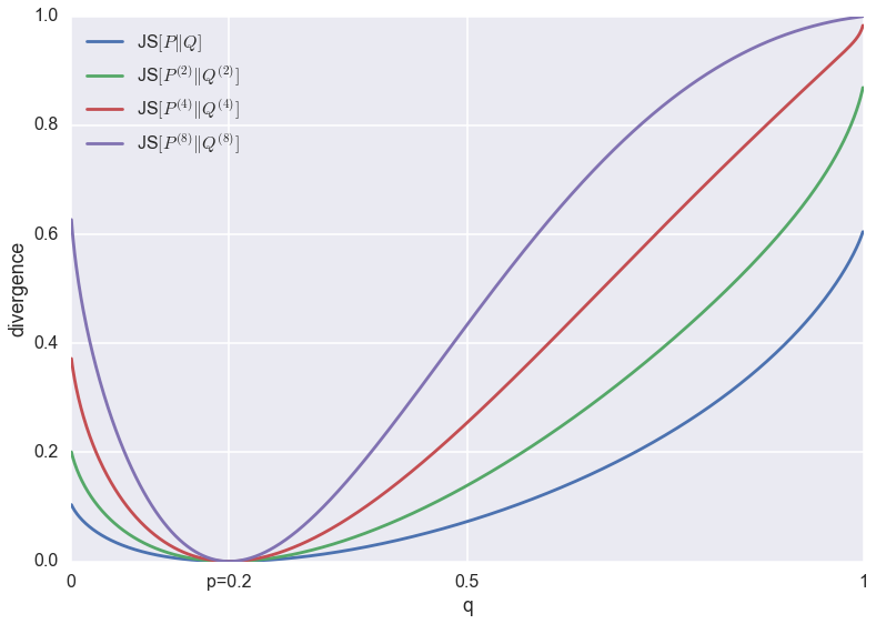
You can see that all divergences have a unique global minimum around $p=q=0.2$. However, their behaviour at the tails changes as the minibatch-size increases. This change in behaviour is due to saturation: JS divergence is upper bounded by $1$, which corresponds to 1 bit of information. If I continued increasing the minibatch-size (which would blow up the memory footprint of my super-naive script), eventually the divergence would reach $1$ almost everywhere except for a dip down to $0$ around $p=q=0.2$.

Below are the same divergences normalised to be roughly the same scale.

![](http://www.inference.vc/content/images/2016/06/Rle8idcTS3gAAAABJRU5ErkJggg--.png)

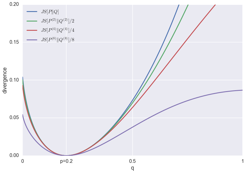
The problem of GANs that minibatch discrimination was meant to fix is that it favours low-entropy solutions. In this plot, this would correspond to the $q<0.1$ regime. You can argue that as the batch-size increases, the relative penalty for low-entropy approximations $q<0.1$ do indeed decrease when compared to completely wrong solutions $q>0.5$. However, the effect is pretty subtle.

Bonus track: adversarial preference loss

In this context, I also revisited the adversarial preference loss. Here, the discriminator receives two inputs $x_1$ and $x_2$ (one synthetic, one real) and it has to decide which one was real.

This algorithm, too, can be related to the minibatch discrimination approach, as it minimises the following divergence:

$$ d(P,Q) = d(P\times Q\|Q\times P), 
$$

where $P\times Q(x_1,x_2) = P(x_1)Q(x_2)$. Again, if $d$ is the $KL$ divergence, the training objective boils down to the same thing as the original GAN. However, if $d$ is the JS divergence, we will end up minimising something weird, $\operatorname{JS}[Q\times P\| P\times Q]$

- I give an overview of the paper which proposes an exponential schedule of dilated convolutional layers as a way to combine local and global knowledge
- I point out the connection between 2D dilated convolutions and Kronecker products
- cascades of exponentially dilated convolutions - as proposed in the paper - can be thought of as parametrising a large convolution kernel as a Kronecker product of small kernels
- the relationship to Kronecker factorisation only holds under particular assumptions, in this sense cascades of exponenetially diluted convolutions are a generalisation of the Kronecker layer (Zhou et al. 2015)
- I note that dilated convolutions are equivariant under image translation, a property that other multi-scale architectures often violate.

#### Background

The key application the dilated convolution authors have in mind is dense prediction: vision applications where the predicted object that has similar size and structure to the input image. For example, semantic segmentation with one label per pixel; image super-resolution, denoising, demosaicing, bottom-up saliency, keypoint detection, etc.

In many such applications one wants to integrate information from different spatial scales and balance two properties:

1. local, pixel-level accuracy, such as precise detection of edges, and
2. integrating knowledge of the wider, global context

To address this problem, people often use some kind of multi-scale convolutional neural networks, which often relies on spatial pooling. Instead the authors here propose using layers dilated convolutions, which allow us to address the multi-scale problem efficiently without increasing the number of parameters too much.

#### Dilated Convolutions

It's perhaps useful to first note why vanilla convolutions struggle to integrate global context. Consider a purely convolutional network composed of layers of $k\times k$ convolutions, without pooling. It is easy to see that size of the receptive field of each unit - the block of pixels which can influence its activation - is $l*(k-1)+k$, where $l$ is the layer index. So the effective receptive field of units can only grow linearly with layers. This is very limiting, especially for high-resolution input images.

Dilated convolutions to the rescue! The dilated convolution between signal $f$ and kernel $k$ and dilution factor $l$ is defined as:

$$ \left(k \ast_{l} f\right)_t = \sum_{\tau=-\infty}^{\infty} k_\tau \cdot f_{t - l\tau} $$

Note that I'm using slightly different notation than the authors. The above formula differs from vanilla convolution in last subscript $f_{t - l\tau}$. For plain old convolution this would be $f_{t - \tau}$. In the dilated convolution, the kernel only touches the signal at every $l^{th}$ entry. This formula applies to a 1D signal, but it can be straightforwardly extended to 2D convolutions.

The authors then build a network out of multiple layers of diluted convolutions, where the dilation factor $l$ increases exponentially at each layer. When you do that, even though the number of parameters grows only linearly with layers, the effective receptive field of units grows exponentially with layer depth. This is illustrated in the figure below:

![](http://www.inference.vc/content/images/2016/05/Screen-Shot-2016-05-12-at-09-47-12.png)

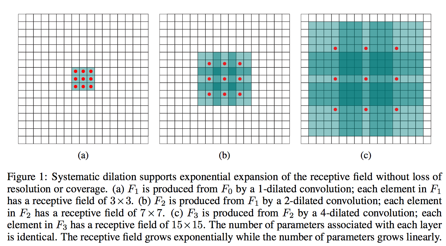
What this figure doesn't really show is the parameter sharing and parameter dependencies across the receptive field (frankly, it's pretty hard to visualise exactly with more than 2 layers). The receptive field grows at a faster rate than the number of parameters, and it is obvious that this can only be achieved by introducing additional constraints on the parameters across the receptive field. The network won't be able to learn arbitrary receptive field behaviours, so one question is, how severe is that restriction?

#### Relationship to Kronecker Products

To me this whole dilated convolution paper cries Kronecker product, although this connection is never made in the paper itself. It's easy to see that a 2D dilated convolution with matrix/filter $K$ is the same as vanilla convolution with a diluted filter $\hat{K}_{l}$ which can be represented as the following Kronecker product:

$$ \hat{K}_l = K \otimes \begin{bmatrix} 1 & 0 & 0 & 0 & 0 \\ 
0 & 0 & \ddots & & 0 \\ 
0 & \ddots & \ddots & \ddots & \\ 
0 & & \ddots & \ddots & 0 \\ 
0 & 0 & 0 & 0 & 0 
\end{bmatrix} $$

Using this, and properties of convolutions and Kronecker products (I suggest beginners to make extensive use of the matrix cookbook) we can even understand something about exponentially iterated dilated convolutions.

Let's assume we apply several layers of dilated convolutions, without nonlinearity, as in Equation 3 of the paper. For simplicity, I assume that that all convolution kernels $K_l, L=1\ldots L$ are $a\times a$ in size, the dilation factor at layer $l$ is $a^{l}$, and we only have a single channel throughout ($C=1$). In this case we can show that:

$$ F_{L+1} = K_L \ast_{a^L} \left( K_{L-1} \ast_{a^{(L-1)}} \left( \cdots K_1 \ast_{a} \left( K_0 \ast F_0 \right) \cdots \right) \right) = \left( K_L \otimes K_{L-1} \otimes \cdots \otimes K_{0} \right) \ast F_0 
$$

The left-hand side of this equation is the same construction as in Equation 3 in the paper, but expanded. The right hand side is a single vanilla convolution, but with a convolution kernel that is constructed as the Kronecker product of all the $a\times a$ kernels $K_l$.

It turns out Kronecker-factored parametrisations of convolution tensors are already used in CNNs, a quick googling revealed this paper:

Shuchang Zhou, Jia-Nan Wu, Yuxin Wu, Xinyu Zhou (2015) Exploiting Local Structures with the Kronecker Layer in Convolutional Networks
What can Kronecker-factored filters represent?

Let's look at what kind of kernels can we represent with Kronecker products, and hence what behaviour should we expect from dilated convolutions. Here are a few examples of $27\times 27$ kernels that result from taking the Kronecker product of three random $3\times 3$ kernels:

![](http://www.inference.vc/content/images/2016/05/VzORx0FEfAAAAAElFTkSuQmCC.png)

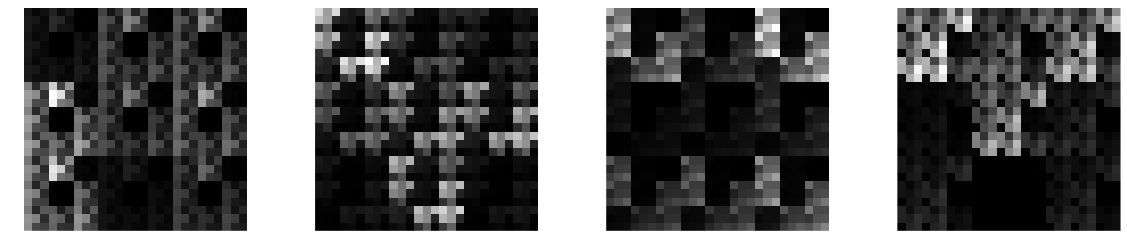
These look somehow natural, at least to me. They look like pretty plausible texture patches taken from some pixellated video game. You will notice the repeated patterns and the hierarchical structure. Indeed, we can draw cool self-similar fractal-like filters if we keep taking the Kronecker product of the same kernel with itself, some examples of such random fractals:

![](http://www.inference.vc/content/images/2016/05/YSJIkSZIkLYw3bCRJkiRJkhbGGzaSJEmSJEkL8zeSmRmMrhHPQgAAAABJRU5ErkJggg--.png)

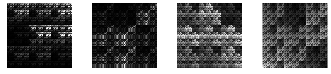
I would say these kernels are not entirely unreasonable for a ConvNet, and if you allow for multiple channels ($C>1$) they can represent pretty nice structured patterns and shapes with reasonable number of parameters.

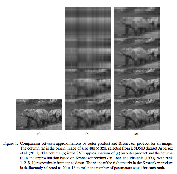
Compare these filters to another common technique for reducing parameters of convolution tensors: low-rank decompositions (see e.g. Lebedev et al, 2014). Spatially, a low-rank approximation to a square 2D convolution filter can be understood as subsequently applying two smaller rectangular filters: one with a limited horizontal extent and one with limited vertical extent. Here are a few random samples of $27\times 27$ filters with a rank of 1. These can be represented using the same number of parameters (27) as the Kronecker samples above.



To me, these don't look so natural. Notice also that for low-rank representations the number of parameters has to scale linearly with the spatial extent of the filter, whereas this scaling can be logarithmic if we use a Kronecker parametrisation. This is the real deal when using Kronecker products or dilated convolutions.

Here is another cool illustration of the naturalness of the Kronecker approximation, taken out of the Kronecker layer paper:

![](http://www.inference.vc/content/images/2016/05/Screen-Shot-2016-05-12-at-14-58-33.png)

So in general, parametrising convolution kernels as Kronecker-products seems like a pretty good idea. The dilated convolutions paper presents a more flexible approach than just Kronecker-factors. Firstly, you can add nonlinearities after each layer of dilated convolution, which would now be different from Kronecker products. Secondly, the Kronecker analogy only holds if the dilation factor and the kernel size are the same. In the paper the authors used a kernel size of $3$ and dilation factor of $2$.

#### Final note on translational equivariance

One desirable property of convolutions is that they are translationally equivariant: if you shift the input image by any amount, the output remains the same, shifted by the same amount. This is a very useful inductive bias/prior assumtion to use in a dense prediction task.

One way to introduce multiscale thinking to ConvNets is to use architectures that look like the figure below: we first decrease the spatial extent of feature-maps via pooling, then grow them back again via unpooling/deconvolution. Additional shortcut connections ensure that pixel-level local accuracy can be retained. The example below is from the SegNet paper, but there are multiple other papers such as this one on recombinator networks.

![](http://www.inference.vc/content/images/2016/05/conv-deconv.png)

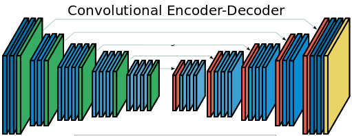
However, as soon as you include spatial pooling, the translational equivariance property of the whole network might break. For example the SegNet above is not translationally equivariant anymore: the network's predictions are sensitive to small, single-pixel shifts to the input image, which is undesirable. Thankfully, layers of dilated convolutions are still translationally equivariant, which is a good thing.

#### Summary

This dilated convolutions idea is pretty cool, and I think these papers are just scratching the surface of this topic. The dilated convolution architecture generalises Kronecker-factored convolutional filters, it allows for very large receptive fields while only growing the number o

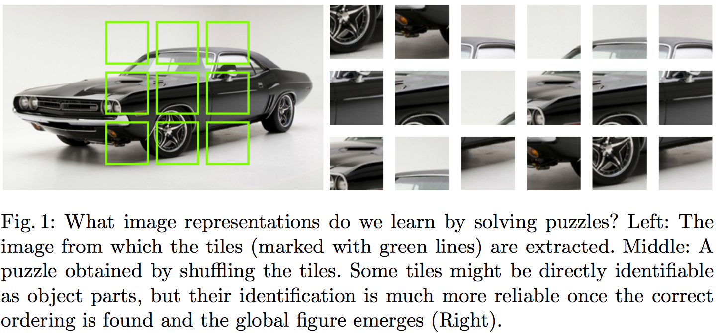
The core idea behind this paper is powerfully simple. The goal is to learn useful representations from unlabelled data, useful in the sense of helping supervised object classification. This paper does this by chopping up images into a set of little jigsaw puzzle, scrambling the pieces, and asking a deep neural network to learn to reassemble them in the correct constellation. A picture is worth a thousand words, so here is Figure 1 taken from the paper explaining this visually:

![](http://www.inference.vc/content/images/2016/04/Screen-Shot-2016-04-25-at-08-26-45-1.png)

#### Summary of this note:

- I note the similarities to denoising autoencoders, which motivate my question: "Can this method equivalently represent the data generating distribution?"
- I consider a toy example with just two jigsaw pieces, and consider using an objective like this to fit a generative model $Q$ to data
- I show how the jigsaw puzzle training procedure corresponds to minimising a difference of KL divergences
- Conclude that the algorithm ignores some aspects of the data generating distribution, and argue that in this case it can be a good thing

#### What does this learn do?

This idea seems to make a lot of sense. But to me, one interesting question is the following:

`What does a network trained to solve jigsaw puzzle learn about the data generating distribution?`

#### Motivating example: denoising autoencoders

At one level, this jigsaw puzzle approach bears similarities to denoising autoencoders (DAEs): both methods are self-supervised: they take an unlabelled data and generate a synthetic supervised learning task. You can also interpret solving jigsaw puzzles as a special case 'undoing corruption' thus fitting a more general definition of autoencoders (Bengio et al, 2014).

DAEs have been shown to be related to score matching (Vincent, 2000), and that they learn to represent gradients of the log-probability-density-function of the data generating distribution (Alain et al, 2012). In this sense, autoencoders equivalently represent a complete probability distribution up to normalisation. This concept is also exploited in Harri Valpola's work on ladder networks (Rasmus et al, 2015)

So I was curious if I can find a similar neat interpretation of what really is going on in this jigsaw puzzle thing. If you equivalently represent all aspects of a probability distribution this way? Are there aspects that this representation ignores? Would it correspond to a consistent denisty estimation/generative modelling method in any sense? Below is my attempt to figure this out.

#### A toy case with just two jigsaw pieces

To simplify things, let's just consider a simpler jigsaw puzzle problem with just two jigsaw positions instead of 9, and in such a way that there are no gaps between puzzle pieces, so image patches (now on referred to as data $x$) can be partitioned exactly into pieces.

Let's assume our datapoints $x^{(n)}$ are drawn i.i.d. from an unknown distribution $P$, and that $x$ can be partitioned into two chunks $x_1$ and $x_2$ of equivalent dimensionality, such that $x=(x_1,x_2)$ by definition. Let's also define the permuted/scrambled version of a datapoint $x$ as $\hat{x}:=(x_2,x_1)$.

The jigsaw puzzle problem can be formulated in the following way: we draw a datapoint $x$ from $P$. We also independently draw a binary 'label' $y$ from a Bernoulli($\frac{1}{2}$) distribution, i.e. toss a coin. If $y=1$ we set $z=x$ otherwise $z=\hat{x}$.

Our task is to build a predictior, $f$, which receives as input $z$ and infers the value of $y$ (outputs the probability that its value is $1$). In other words, $f$ tries to guess the correct ordering of the chunks that make up the randomly scrambled datapoint $z$, thereby solving the jigsaw puzzle. The accuracy of the predictor is evaluated using the log-loss, a.k.a. binary cross-entropy, as it is common in binary classification problems:

$$ \mathcal{L}(f) = - \frac{1}{2} \mathbb{E}_{x\sim P} \left[\log f(x) + \log (1 - f(\hat{x}))\right] $$

Let's consider the case when we express the predictor $f$ in terms of a generative model $Q$ of $x$. $Q$ is an approximation to $P$, and has some parameters $\theta$ which we can tweak. For a given $\theta$, the posterior predictive distribution of $y$ takes the following form:

$$ f(z,\theta) := Q(y=1\vert z;\theta) = \frac{Q(z;\theta)}{Q(z;\theta) + Q(\hat{z};\theta)}, 
$$

where $\hat{z}$ denotes the scrambled/permuted version of $z$. Notice that when $f$ is defined this way the following property holds:

$$ 1 - f(\hat{x};\theta) = f(x;\theta), 
$$

so we can simplify the expression for the log-loss to finally obtain:

\begin{align} \mathcal{L}(\theta) &= - \mathbb{E}_{x \sim P} \log Q(x;\theta) + \mathbb{E}_{x \sim P} \log [Q(x;\theta) + Q(\hat{x};\theta)]\\ &= \operatorname{KL}[P\|Q_{\theta}] - \operatorname{KL}\left[P\middle\|\frac{Q_{\theta}(x)+Q_{\theta}(\hat{x})}{2}\right] + \log(2) \end{align}

So we already see that using the jigsaw objective to train a generative model reduces to minimising the difference between two KL divergences. It's also possible to reformulate the loss as:

$$ \mathcal{L}(\theta) = \operatorname{KL}[P\|Q_{\theta}] - \operatorname{KL}\left[\frac{P(x) + P(\hat{x})}{2}\middle\|\frac{Q_{\theta}(x)+Q_{\theta}(\hat{x})}{2}\right] - \operatorname{KL}\left[P\middle\|\frac{P(x) + P(\hat{x})}{2}\right] + \log(2) $$

Let's look at what the different terms do:

- The first term is the usual KL divergence that would correspond to maximum likelihood. So it just tries to make $Q$ as close to $P$ as possible.
- The second term is a bit weird, particularly as comes into the formula with a negative sign. The KL divergence is $0$ if $Q$ and $P$ define the distribution over the set of jigsaw pieces ${x_1,x_2}$. Notice, I used set notation here, so the ordering does not matter. In a way this term tells the loss function: don't bother modelling what the jigsaw pieces are, only model how they fit together.
- The last terms are constant wrt. $\theta$ so we don't need to worry about them.

#### Not a proper scoring rule (and it's okay)

From the formula above it is clear that the jigsaw training objective wouldn't be a proper scoring rule, as it is not uniquely minimised by $Q=P$ in all cases. Here are two counterexamples where the objective fails to capture all aspects of $P$:

Consider the case when $P=\frac{P(x) + P(\hat{x})}{2}$, that is, when $P$ is completely insensitive to the ordering of jigsaw pieces. As long as $Q$ also has this property $Q = \frac{Q(x) + Q(\hat{x})}{2}$, all KL divergences are $0$ and the jigsaw objective is constant with respect $\theta$. Indeed, it is impossible in this case for any classifier to surpass chance level in the jigsaw problem.

Another simple example to consider is a two-dimensional binary $P$. Here, the jigsaw objective only cares about the value of $Q(0,1)$ relative to $Q(1,0)$, but completely insensitive to $Q(1,1)$ and $Q(0,0)$. In other words, we don't really care how often $0$s and $1$s appear, we just want to know which one is likelier to be on the left or the right side.

This is all fine because we don't use this technique for generative modelling. We want to use it for representation learning, so it's okay to ignore some aspects of $P$.

#### Representation learning

I think this method seems like a really promising direction for unsupervised representation learning. In my mind representation learning needs either:

- strong prior assumptions about what variables/aspects of data are behaviourally relevant, or relevant to the tasks we want to solve with the representations.
- at least a little data in a semi-supervised setting to inform us about what is relevant and what is not.

Denoising autoencoders (with L2 reconstruction loss) and maximum likelihood training try to represent all aspects of the data generating distribution, down to pixel level. We can encode further priors in these models in various ways, either by constraining the network architecture or via probabilistic priors over latent variables.

The jigsaw method encodes prior assumptions into the training procedure: that the structure of the world (relative position of parts) is more important to get right than the low-level appearance of parts. This is probably a fair assumption.