This paper presents a method to train a neural network to make predictions for *counterfactual* questions. In short, such questions are questions about what the result of an intervention would have been, had a different choice for the intervention been made (e.g. *Would this patient have lower blood sugar had she received a different medication?*).

One approach to tackle this problem is to collect data of the form $(x_i, t_i, y_i^F)$ where $x_i$ describes a situation (e.g. a patient), $t_i$ describes the intervention made (in this paper $t_i$ is binary, e.g. $t_i = 1$ if a new treatment is used while $t_i = 0$ would correspond to using the current treatment) and $y_i^F$ is the factual outcome of the intervention $t_i$ for $x_i$. From this training data, a predictor $h(x,t)$ taking the pair $(x_i, t_i)$ as input and outputting a prediction for $y_i^F$ could be trained. 

From this predictor, one could imagine answering counterfactual questions by feeding $(x_i, 1-t_i)$ (i.e. a description of the same situation $x_i$ but with the opposite intervention $1-t_i$) to our predictor and comparing the prediction $h(x_i, 1-t_i)$ with $y_i^F$. This would give us an estimate of the change in the outcome, had a different intervention been made, thus providing an answer to our counterfactual question.

The authors point out that this scenario is related to that of domain adaptation (more specifically to the special case of covariate shift) in which the input training distribution (here represented by inputs $(x_i,t_i)$) is different from the distribution of inputs that will be fed at test time to our predictor (corresponding to the inputs $(x_i, 1-t_i)$). If the choice of intervention $t_i$ is evenly spread and chosen independently from $x_i$, the distributions become the same. However, in observational studies, the choice of $t_i$ for some given $x_i$ is often not independent of $x_i$ and made according to some unknown policy. This is the situation of interest in this paper.

Thus, the authors propose an approach inspired by the domain adaptation literature. Specifically, they propose to have the predictor $h(x,t)$ learn a representation of $x$ that is indiscriminate of the intervention $t$ (see Figure 2 for the proposed neural network architecture). Indeed, this is a notion that is [well established][1] in the domain adaptation literature and has been exploited previously using regularization terms based on [adversarial learning][2] and [maximum mean discrepancy][3]. In this paper, the authors used instead a regularization (noted in the paper as $disc(\Phi_{t=0},\Phi_ {t=1})$) based on the so-called discrepancy distance of [Mansour et al.][4], adapting its use to the case of a neural network. 

As an example, imagine that in our dataset, a new treatment ($t=1$) was much more frequently used than not ($t=0$) for men. Thus, for men, relatively insufficient evidence for counterfactual inference is expected to be found in our training dataset. Intuitively, we would thus want our predictor to not rely as much on that "feature" of patients when inferring the impact of the treatment. 

In addition to this term, the authors also propose incorporating an additional regularizer where the prediction $h(x_i,1-t_i)$ on counterfactual inputs is pushed to be as close as possible to the target $y_{j}^F$ of the observation $x_j$ that is closest to $x_i$ **and** actually had the counterfactual intervention $t_j = 1-t_i$. 

The paper first shows a bound relating the counterfactual generalization error to the discrepancy distance. Moreover, experiments simulating counterfactual inference tasks are presented, in which performance is measured by comparing the predicted treatment effects (as estimated by the difference between the observed effect $y_i^F$ for the observed treatment and the predicted effect $h(x_i, 1-t_i)$ for the opposite treatment) with the real effect (known here because the data is simulated). The paper shows that the proposed approach using neural networks outperforms several baselines on this task.

**My two cents**

The connection with domain adaptation presented here is really clever and enlightening. This sounds like a very compelling approach to counterfactual inference, which can exploit a lot of previous work on domain adaptation.

The paper mentions that selecting the hyper-parameters (such as the regularization terms weights) in this scenario is not a trivial task. Indeed, measuring performance here requires knowing the true difference in intervention outcomes, which in practice usually cannot be known (e.g. two treatments usually cannot be given to the same patient once). In the paper, they somewhat "cheat" by using the ground truth difference in outcomes to measure out-of-sample performance, which the authors admit is unrealistic. Thus, an interesting avenue for future work would be to design practical hyper-parameter selection procedures for this scenario. I wonder whether the *reverse cross-validation* approach we used in our work on our adversarial approach to domain adaptation (see [Section 5.1.2][5]) could successfully be used here.

Finally, I command the authors for presenting such a nicely written description of counterfactual inference problem setup in general, I really enjoyed it!

[1]: https://papers.nips.cc/paper/2983-analysis-of-representations-for-domain-adaptation.pdf
[2]: http://arxiv.org/abs/1505.07818
[3]: http://ijcai.org/Proceedings/09/Papers/200.pdf
[4]: http://www.cs.nyu.edu/~mohri/pub/nadap.pdf
[5]: http://arxiv.org/pdf/1505.07818v4.pdf#page=16

This paper was published after the 2015 Duvenaud et al paper proposing a differentiable alternative to circular fingerprints of molecules: substituting out exact-match random hash functions to identify molecular structures with learned convolutional-esque kernels. As far as I can tell, the Duvenaud paper was the first to propose something we might today recognize as graph convolutions on atoms. I hoped this paper would build on that one, but it seems to be coming from a conceptually different direction, and it seems like it was more or less contemporaneous, for all that it was released later. 

This paper introduces a structure that allows for more explicit message passing along bonds, by calculating atom features as a function of their incoming bonds, and then bond features as a function of their constituent atoms, and iterating this procedure, so information from an atom can be passed into a bond, then, on the next iteration, pulled in by another atom on the other end of that bond, and then pulled into that atom's bonds, and so forth. This has the effect of, similar to a convolutional or recurrent network, creating representations for each atom in the molecular graph that are informed by context elsewhere in the graph, to different degrees depending on distance from that atom. 

More specifically, it defines: 

- A function mapping from a prior layer atom representation to a subsequent layer atom representation, taking into account only information from that atom (Atom to Atom)
- A function mapping from a prior layer bond representation (indexed by the two atoms on either side of the bond), taking into account only information from that bond at the prior layer (Bond to Bond)
- A function creating a bond representation by applying a shared function to the atoms at either end of it, and then combining those representations with an aggregator function (Atoms to Bond)
- A function creating an atom representation by applying a shared function all the bonds that atom is a part of, and then combining those results with an aggregator function (Bonds to Atom)

At the top of this set of layers, when each atom has had information diffused into it by other parts of the graph, depending on the network depth, the authors aggregate the per-atom representations into histograms (basically, instead of summing or max-pooling feature-wise, creating course distributions of each feature), and use that for supervised tasks. 

One frustration I had with this paper is that it doesn't do a great job of highlighting its differences with and advantages over prior work; in particular, I think it doesn't do a very good job arguing that its performance is superior to the earlier Duvenaud work. That said, for all that the presentation wasn't ideal, the idea of message-passing is an important one in graph convolutions, and will end up becoming more standard in later works.

#### Summary of this post: 

* an overview the motivation behind adversarial autoencoders and how they work * a discussion on whether the adversarial training is necessary in the first place. tl;dr: I think it's an overkill and I propose a simpler method along the lines of kernel moment matching.

#### Adversarial Autoencoders

Again, I recommend everyone interested to read the actual paper, but I'll attempt to give a high level overview the main ideas in the paper. I think the main figure from the paper does a pretty good job explaining how Adversarial Autoencoders are trained:

![](http://www.inference.vc/content/images/2016/01/Screen-Shot-2016-01-08-at-14-48-25.png)

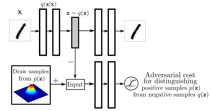
The top part of this image is a probabilistic autoencoder. Given the input $\mathbf{x}$, some latent code $\mathbf{z}$ is generated by sampling from an encoding distribution $q(\mathbf{z}\vert\mathbf{x})$. This distribution is typically modeled as the output a deep neural network. In normal autoencoders this encoder would be deterministic, now we allow it to be probabilistic.

A decoder network is then trained to decode $\mathbf{z}$ and reconstruct the original input $\mathbf{x}$. Of course, reconstruction will not be perfect, but we train the networks to minimise reconstruction error, this is typically just mean squared error.

The reconstruction cost ensures that the encoding process retains information about the input image, but it doesn't enforce anything else about what these latent representations $\mathbf{z}$ should do. In general, their distribution is described as the aggregate posterior $q(\mathbf{z})=\mathbb{E}_\mathbf{x} q(\mathbf{z}\vert\mathbf{x})$. Often, we would like this distribution to match a certain prior $p(\mathbf{z})$. For example. we may want $\mathbf{z}$ to have independent components and Gaussian distributed (nonlinear ICA,PCA). Or we may want to force the latent representations to correspond to discrete class labels, or binary factors. Or we may simply want to ensure there are 'no gaps' in the latent space, and any random $\mathbf{z}$ would lead to a viable sample when squashed through the decoder network.

So there are multiple reasons why one might want to control the aggregate posterior $q(\mathbf{z})$ to match a predefined prior $p(\mathbf{z})$. The authors achieve this by introducing an additional term in the autoencoder loss function, one that measures the divergence between $q$ and $p$. The authors chose to do this via adversarial training: they train a discriminator network that constantly learns to discriminate between real code vectors $\mathbb{z}$ produced by encoding real data, and random code vectors sampled from $p$. If $q$ matches $p$ perfectly, the optimal discriminator network should have a large classification error.

#### Is this an overkill?

My main question about this paper was whether the adversarial cost is really needed here, because I think it's an overkill. Let me explain:

Adversarial training is powerful when all else fails to quantify divergence between complicated, potentially degenerate distributions in high dimensions, such as images or video. Our toolkit for dealing with images is limited, CNNs are the best tool we have, so it makes sense to incorporate them in training generative models for images. GANs - when applied directly to images - are a great idea.

However, here adversarial training is applied to an easier problem: to quantify the divergence between a simple, fixed prior (e.g. Gaussian) and an empirical distribution of latents. The latent space is usually lower-dimensional, distributions better behaved. Therefore, matching to $p(\mathbf{z})$ in latent space should be considerably easier than matching distributions over images.

Adversarial training makes no assumptions about the distributions compared, other than sampling from them. This comes very handy when both $p$ and $q$ are nasty such as in the generative adversarial network scenario: there, $p$ is the distribution of natural images, $q$ is a super complicated, degenerate distribution produced by squashing noise through a deep convnet. The price we pay for this flexibility is this: when $p$ or $q$ are actually easy to work with, adversarial training cannot exploit that, it still has to sample. (it would be interesting to see if expectations over $p(\mathbf{z})$ could be computed analytically). So even though in this work $p$ is as simple as a mixture of ten 2D Gaussians, we need to approximate everything by drawing samples.

#### Other things might work: kernel moment matching

Why can’t one use easier divergences? For example, I think moment matching based on kernel MMD would work brilliantly in this scenario. It would have the following advantages over the adversarial cost.

- closed form expressions: Depending on the choice of the prior $p(\mathbf{z})$ and kernel used in MMD, the expectations over $p$ may be available in closed form, without sampling. So for example if we use a squared exponential kernel and a mixture of Gaussians as $p$, the divergence from $p$ can be precomputed in closed form that is easy to evaluate.

- no nasty inner loop: Adversarial training requires the discriminator network to be reoptimised every time the generative model changes. So we end up with a gradient descent in the inner loop of a gradient descent, which is anything but nice to work with. This is why it takes so long to get it working, the whole thing is pretty unstable. In contrast, to evaluate MMD, the inner loop is not needed. In fact, MMD can also be thought of as the solution to a convex maximisation problem, but via the kernel trick the maximum has a closed form solution.

- the problem is well suited for MMD: because the distributions are smooth, and the space is nice and low-dimensional, MMD might work very well. Kernel-based methods struggle with complicated manifold-like structure of natural images, so I wouldn't expect MMD to be competitive with adversarial training if it is applied directly in the image space. Therefore, I actually prefer generative adversarial networks to generative moment matching networks. However, here we have an easier problem, simpler space, simpler distributions where MMD shines, and adversarial training is just not needed.

The main contribution of [Asynchronous Methods for Deep Reinforcement Learning](https://arxiv.org/pdf/1602.01783v1.pdf) by Mnih et al. is a ligthweight framework for reinforcement learning agents. 

They propose a training procedure which utilizes asynchronous gradient decent updates from multiple agents at once. Instead of training one single agent who interacts with its environment, multiple agents are interacting with their own version of the environment simultaneously.

After a certain amount of timesteps, accumulated gradient updates from an agent are applied to a global model, e.g. a Deep Q-Network. These updates are asynchronous and lock free. 

Effects of training speed and quality are analyzed for various reinforcement learning methods. No replay memory is need to decorrelate successive game states, since all agents are already exploring different game states in real time. Also, on-policy algorithms like actor-critic can be applied.

They show that asynchronous updates have a stabilizing effect on policy and value updates. Also, their best method, an asynchronous variant of actor-critic, surpasses the current state-of-the-art on the Atari domain while training for half the time on a single multi-core CPU instead of a GPU.

Originally posted on my Github [paper-notes](https://github.com/karpathy/paper-notes/blob/master/matching_networks.md) repo.

# Matching Networks for One Shot Learning

By DeepMind crew: **Oriol Vinyals, Charles Blundell, Timothy Lillicrap, Koray Kavukcuoglu, Daan Wierstra**

This is a paper on **one-shot** learning, where we'd like to learn a class based on very few (or indeed, 1) training examples. E.g. it suffices to show a child a single giraffe, not a few hundred thousands before it can recognize more giraffes.

This paper falls into a category of *"duh of course"* kind of paper, something very interesting, powerful, but somehow obvious only in retrospect. I like it.

Suppose you're given a single example of some class and would like to label it in test images.

- **Observation 1**: a standard approach might be to train an Exemplar SVM for this one (or few) examples vs. all the other training examples - i.e. a linear classifier. But this requires optimization.
- **Observation 2:** known non-parameteric alternatives (e.g. k-Nearest Neighbor) don't suffer from this problem. E.g. I could immediately use a Nearest Neighbor to classify the new class without having to do any optimization whatsoever. However, NN is gross because it depends on an (arbitrarily-chosen) metric, e.g. L2 distance. Ew.
- **Core idea**: lets train a fully end-to-end nearest neighbor classifer!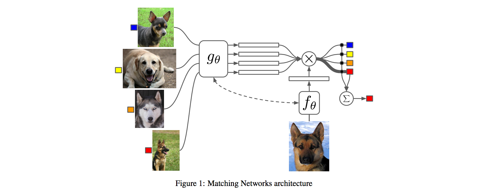![Screen Shot 2016-08-07 at 10.08.44 PM](https://raw.githubusercontent.com/karpathy/paper-notes/master/img/matching_networks/Screen%20Shot%202016-08-07%20at%2010.08.44%20PM.png)

## The training protocol

As the authors amusingly point out in the conclusion (and this is the *duh of course* part), *"one-shot learning is much easier if you train the network to do one-shot learning"*. Therefore, we want the test-time protocol (given N novel classes with only k examples each (e.g. k = 1 or 5), predict new instances to one of N classes) to exactly match the training time protocol.

To create each "episode" of training from a dataset of examples then:

1. Sample a task T from the training data, e.g. select 5 labels, and up to 5 examples per label (i.e. 5-25 examples).
2. To form one episode sample a label set L (e.g. {cats, dogs}) and then use L to sample the support set S and a batch B of examples to evaluate loss on.

The idea on high level is clear but the writing here is a bit unclear on details, of exactly how the sampling is done.

## The model

I find the paper's model description slightly wordy and unclear, but basically we're building a **differentiable nearest neighbor++**. The output \hat{y} for a test example \hat{x} is computed very similar to what you might see in Nearest Neighbors:![Screen Shot 2016-08-07 at 11.14.26 PM](https://raw.githubusercontent.com/karpathy/paper-notes/master/img/matching_networks/Screen%20Shot%202016-08-07%20at%2011.14.26%20PM.png)
where **a** acts as a kernel, computing the extent to which \hat{x} is similar to a training example x_i, and then the labels from the training examples (y_i) are weight-blended together accordingly. The paper doesn't mention this but I assume for classification y_i would presumbly be one-hot vectors.

Now, we're going to embed both the training examples x_i and the test example \hat{x}, and we'll interpret their inner products (or here a cosine similarity) as the "match", and pass that through a softmax to get normalized mixing weights so they add up to 1. No surprises here, this is quite natural:

![Screen Shot 2016-08-07 at 11.20.29 PM](https://raw.githubusercontent.com/karpathy/paper-notes/master/img/matching_networks/Screen%20Shot%202016-08-07%20at%2011.20.29%20PM.png)
Here **c()** is cosine distance, which I presume is implemented by normalizing the two input vectors to have unit L2 norm and taking a dot product. I assume the authors tried skipping the normalization too and it did worse? Anyway, now all that's left to define is the function **f** (i.e. how do we embed the test example into a vector) and the function **g** (i.e. how do we embed each training example into a vector?).

**Embedding the training examples.** This (the function **g**) is a bidirectional LSTM over the examples:

 ![Screen Shot 2016-08-07 at 11.57.10 PM](https://raw.githubusercontent.com/karpathy/paper-notes/master/img/matching_networks/Screen%20Shot%202016-08-07%20at%2011.57.10%20PM.png)

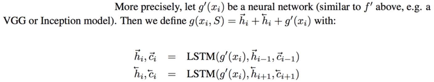
i.e. encoding of i'th example x_i is a function of its "raw" embedding g'(x_i) and the embedding of its friends, communicated through the bidirectional network's hidden states. i.e. each training example is a function of not just itself but all of its friends in the set. This is part of the ++ above, because in a normal nearest neighbor you wouldn't change the representation of an example as a function of the other data points in the training set.

It's odd that the **order** is not mentioned, I assume it's random? This is a bit gross because order matters to a bidirectional LSTM; you'd get different embeddings if you permute the examples. 

**Embedding the test example.** This (the function **f**) is a an LSTM that processes for a fixed amount (K time steps) and at each point also *attends* over the examples in the training set. The encoding is the last hidden state of the LSTM. Again, this way we're allowing the network to change its encoding of the test example as a function of the training examples. Nifty: 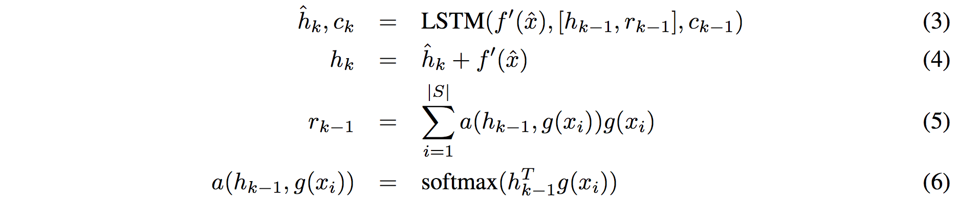![Screen Shot 2016-08-08 at 12.11.15 AM](https://raw.githubusercontent.com/karpathy/paper-notes/master/img/matching_networks/Screen%20Shot%202016-08-08%20at%2012.11.15%20AM.png)

That looks scary at first but it's really just a vanilla LSTM with attention where the input at each time step is constant (f'(\hat{x}), an encoding of the test example all by itself) and the hidden state is a function of previous hidden state but also a concatenated readout vector **r**, which we obtain by attending over the encoded training examples (encoded with **g** from above).

Oh and I assume there is a typo in equation (5), it should say r_k = … without the -1 on LHS. 



## Experiments

**Task**: N-way k-shot learning task. i.e. we're given k (e.g. 1 or 5) labelled examples for N classes that we have not previously trained on and asked to classify new instances into he N classes.

**Baselines:** an "obvious" strategy of using a pretrained ConvNet and doing nearest neighbor based on the codes. An option of finetuning the network on the new examples as well (requires training and careful and strong regularization!).

**MANN** of Santoro et al. [21]: Also a DeepMind paper, a fun NTM-like Meta-Learning approach that is fed a sequence of examples and asked to predict their labels.

**Siamese network** of Koch et al. [11]: A siamese network that takes two examples and predicts whether they are from the same class or not with logistic regression. A test example is labeled with a nearest neighbor: with the class it matches best according to the siamese net (requires iteration over all training examples one by one). Also, this approach is less end-to-end than the one here because it requires the ad-hoc nearest neighbor matching, while here the *exact* end task is optimized for. It's beautiful.



### Omniglot experiments 

### ![Screen Shot 2016-08-08 at 10.21.45 AM](https://github.com/karpathy/paper-notes/raw/master/img/matching_networks/Screen%20Shot%202016-08-08%20at%2010.21.45%20AM.png)

Omniglot of [Lake et al. [14]](http://www.cs.toronto.edu/~rsalakhu/papers/LakeEtAl2015Science.pdf) is a MNIST-like scribbles dataset with 1623 characters with 20 examples each.

Image encoder is a CNN with 4 modules of [3x3 CONV 64 filters, batchnorm, ReLU, 2x2 max pool]. The original image is claimed to be so resized from original 28x28 to 1x1x64, which doesn't make sense because factor of 2 downsampling 4 times is reduction of 16, and 28/16 is a non-integer >1. I'm assuming they use VALID convs?

Results: 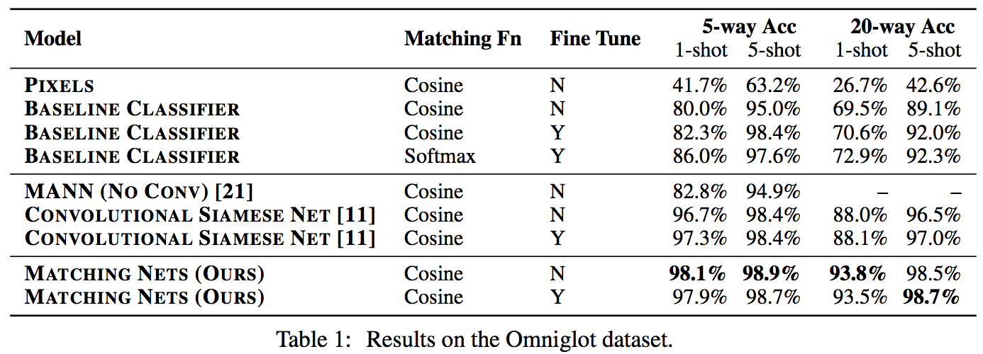![Screen Shot 2016-08-08 at 10.27.46 AM](https://raw.githubusercontent.com/karpathy/paper-notes/master/img/matching_networks/Screen%20Shot%202016-08-08%20at%2010.27.46%20AM.png)

Matching nets do best. Fully Conditional Embeddings (FCE) by which I mean they the "Full Context Embeddings" of Section 2.1.2 instead are not used here, mentioned to not work much better. Finetuning helps a bit on baselines but not with Matching nets (weird).

The comparisons in this table are somewhat confusing:

- I can't find the MANN numbers of 82.8% and 94.9% in their paper [21]; not clear where they come from. E.g. for 5 classes and 5-shot they seem to report 88.4% not 94.9% as seen here. I must be missing something.
- I also can't find the numbers reported here in the Siamese Net [11] paper. As far as I can tell in their Table 2 they report one-shot accuracy, 20-way classification to be 92.0, while here it is listed as 88.1%?
- The results of Lake et al. [14] who proposed Omniglot are also missing from the table. If I'm understanding this correctly they report 95.2% on 1-shot 20-way, while matching nets here show 93.8%, and humans are estimated at 95.5%. That is, the results here appear weaker than those of Lake et al., but one should keep in mind that the method here is significantly more generic and does not make any assumptions about the existence of strokes, etc., and it's a simple, single fully-differentiable blob of neural stuff.

(skipping ImageNet/LM experiments as there are few surprises)

## Conclusions

Good paper, effectively develops a differentiable nearest neighbor trained end-to-end. It's something new, I like it!

A few concerns: 

- A bidirectional LSTMs (not order-invariant compute) is applied over sets of training examples to encode them. The authors don't talk about the order actually used, which presumably is random, or mention this potentially unsatisfying feature. This can be solved by using a recurrent attentional mechanism instead, as the authors are certainly aware of and as has been discussed at length in [ORDER MATTERS: SEQUENCE TO SEQUENCE FOR SETS](https://arxiv.org/abs/1511.06391), where Oriol is also the first author. I wish there was a comment on this point in the paper somewhere.

- The approach also gets quite a bit slower as the number of training examples grow, but once this number is large one would presumable switch over to a parameteric approach.

- It's also potentially concerning that during training the method uses a specific number of examples, e.g. 5-25, so this is the number of that must also be used at test time. What happens if we want the size of our training set to grow online? It appears that we need to retrain the network because the encoder LSTM for the training data is not "used to" seeing inputs of more examples? That is unless you fall back to iteratively subsampling the training data, doing multiple inference passes and averaging, or something like that. If we don't use FCE it can still be that the attention mechanism LSTM can still not be "used to" attending over many more examples, but it's not clear how much this matters. An interesting experiment would be to not use FCE and try to use 100 or 1000 training examples, while only training on up to 25 (with and fithout FCE). Discussion surrounding this point would be interesting.

- Not clear what happened with the Omniglot experiments, with incorrect numbers for [11], [21], and the exclusion of Lake et al. [14] comparison.

- A baseline that is missing would in my opinion also include training of an [Exemplar SVM](https://www.cs.cmu.edu/~tmalisie/projects/iccv11/), which is a much more powerful approach than encode-with-a-cnn-and-nearest-neighbor.

  ​