[link]
Summary by Alexander Jung 8 years ago
* DRAW = deep recurrent attentive writer
* DRAW is a recurrent autoencoder for (primarily) images that uses attention mechanisms.
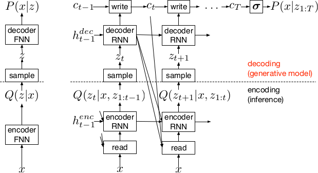
* Like all autoencoders it has an encoder, a latent layer `Z` in the "middle" and a decoder.
* Due to the recurrence, there are actually multiple autoencoders, one for each timestep (the number of timesteps is fixed).
* DRAW has attention mechanisms which allow the model to decide where to look at in the input image ("glimpses") and where to write/draw to in the output image.
* If the attention mechanisms are skipped, the model becomes a simple recurrent autoencoder.
* By training the full autoencoder on a dataset and then only using the decoder, one can generate new images that look similar to the dataset images.

*Basic recurrent architecture of DRAW.*
### How
* General architecture
* The encoder-decoder-pair follows the design of variational autoencoders.
* The latent layer follows an n-dimensional gaussian distribution. The hyperparameters of that distribution (means, standard deviations) are derived from the output of the encoder using a linear transformation.
* Using a gaussian distribution enables the use of the reparameterization trick, which can be useful for backpropagation.
* The decoder receives a sample drawn from that gaussian distribution.
* While the encoder reads from the input image, the decoder writes to an image canvas (where "write" is an addition, not a replacement of the old values).
* The model works in a fixed number of timesteps. At each timestep the encoder performs a read operation and the decoder a write operation.
* Both the encoder and the decoder receive the previous output of the encoder.
* Loss functions
* The loss function of the latent layer is the KL-divergence between that layer's gaussian distribution and a prior, summed over the timesteps.
* The loss function of the decoder is the negative log likelihood of the image given the final canvas content under a bernoulli distribution.
* The total loss, which is optimized, is the expectation of the sum of both losses (latent layer loss, decoder loss).
* Attention
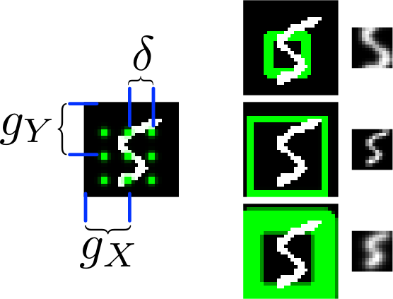
* The selective read attention works on image patches of varying sizes. The result size is always NxN.
* The mechanism has the following parameters:
* `gx`: x-axis coordinate of the center of the patch
* `gy`: y-axis coordinate of the center of the patch
* `delta`: Strides. The higher the strides value, the larger the read image patch.
* `sigma`: Standard deviation. The higher the sigma value, the more blurry the extracted patch will be.
* `gamma`: Intensity-Multiplier. Will be used on the result.
* All of these parameters are generated using a linear transformation applied to the decoder's output.
* The mechanism places a grid of NxN gaussians on the image. The grid is centered at `(gx, gy)`. The gaussians are `delta` pixels apart from each other and have a standard deviation of `sigma`.
* Each gaussian is applied to the image, the center pixel is read and added to the result.

*The basic attention mechanism. (gx, gy) is the read patch center. delta is the strides. On the right: Patches with different sizes/strides and standard deviations/blurriness.*
### Results
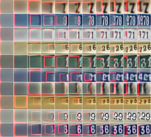
* Realistic looking generated images for MNIST and SVHN.
* Structurally OK, but overall blurry images for CIFAR-10.
* Results with attention are usually significantly better than without attention.
* Image generation without attention starts with a blurry image and progressively sharpens it.

*Using DRAW with attention to generate new SVHN images.*
----------
### Rough chapter-wise notes
* 1. Introduction
* The natural way to draw an image is in a step by step way (add some lines, then add some more, etc.).
* Most generative neural networks however create the image in one step.
* That removes the possibility of iterative self-correction, is hard to scale to large images and makes the image generation process dependent on a single latent distribution (input parameters).
* The DRAW architecture generates images in multiple steps, allowing refinements/corrections.
* DRAW is based on varational autoencoders: An encoder compresses images to codes and a decoder generates images from codes.
* The loss function is a variational upper bound on the log-likelihood of the data.
* DRAW uses recurrance to generate images step by step.
* The recurrance is combined with attention via partial glimpses/foveations (i.e. the model sees only a small part of the image).
* Attention is implemented in a differentiable way in DRAW.
* 2. The DRAW Network
* The DRAW architecture is based on variational autoencoders:
* Encoder: Compresses an image to latent codes, which represent the information contained in the image.
* Decoder: Transforms the codes from the encoder to images (i.e. defines a distribution over images which is conditioned on the distribution of codes).
* Differences to variational autoencoders:
* Encoder and decoder are both recurrent neural networks.
* The encoder receives the previous output of the decoder.
* The decoder writes several times to the image array (instead of only once).
* The encoder has an attention mechanism. It can make a decision about the read location in the input image.
* The decoder has an attention mechanism. It can make a decision about the write location in the output image.
* 2.1 Network architecture
* They use LSTMs for the encoder and decoder.
* The encoder generates a vector.
* The decoder generates a vector.
* The encoder receives at each time step the image and the output of the previous decoding step.
* The hidden layer in between encoder and decoder is a distribution Q(Zt|ht^enc), which is a diagonal gaussian.
* The mean and standard deviation of that gaussian is derived from the encoder's output vector with a linear transformation.
* Using a gaussian instead of a bernoulli distribution enables the use of the reparameterization trick. That trick makes it straightforward to backpropagate "low variance stochastic gradients of the loss function through the latent distribution".
* The decoder writes to an image canvas. At every timestep the vector generated by the decoder is added to that canvas.
* 2.2 Loss function
* The main loss function is the negative log probability: `-log D(x|ct)`, where `x` is the input image and `ct` is the final output image of the autoencoder. `D` is a bernoulli distribution if the image is binary (only 0s and 1s).
* The model also uses a latent loss for the latent layer (between encoder and decoder). That is typical for VAEs. The loss is the KL-Divergence between Q(Zt|ht_enc) (`Zt` = latent layer, `ht_enc` = result of encoder) and a prior `P(Zt)`.
* The full loss function is the expection value of both losses added up.
* 2.3 Stochastic Data Generation
* To generate images, samples can be picked from the latent layer based on a prior. These samples are then fed into the decoder. That is repeated for several timesteps until the image is finished.
* 3. Read and Write Operations
* 3.1 Reading and writing without attention
* Without attention, DRAW simply reads in the whole image and modifies the whole output image canvas at every timestep.
* 3.2 Selective attention model
* The model can decide which parts of the image to read, i.e. where to look at. These looks are called glimpses.
* Each glimpse is defined by its center (x, y), its stride (zoom level), its gaussian variance (the higher the variance, the more blurry is the result) and a scalar multiplier (that scales the intensity of the glimpse result).
* These parameters are calculated based on the decoder output using a linear transformation.
* For an NxN patch/glimpse `N*N` gaussians are created and applied to the image. The center pixel of each gaussian is then used as the respective output pixel of the glimpse.
* 3.3 Reading and writing with attention
* Mostly the same technique from (3.2) is applied to both reading and writing.
* The glimpse parameters are generated from the decoder output in both cases. The parameters can be different (i.e. read and write at different positions).
* For RGB the same glimpses are applied to each channel.
* 4. Experimental results
* They train on binary MNIST, cluttered MNIST, SVHN and CIFAR-10.
* They then classfiy the images (cluttered MNIST) or generate new images (other datasets).
* They say that these generated images are unique (to which degree?) and that they look realistic for MNIST and SVHN.
* Results on CIFAR-10 are blurry.
* They use binary crossentropy as the loss function for binary MNIST.
* They use crossentropy as the loss function for SVHN and CIFAR-10 (color).
* They used Adam as their optimizer.
* 4.1 Cluttered MNIST classification
* They classify images of cluttered MNIST. To do that, they use an LSTM that performs N read-glimpses and then classifies via a softmax layer.
* Their model's error rate is significantly below a previous non-differentiable attention based model.
* Performing more glimpses seems to decrease the error rate further.
* 4.2 MNIST generation
* They generate binary MNIST images using only the decoder.
* DRAW without attention seems to perform similarly to previous models.
* DRAW with attention seems to perform significantly better than previous models.
* DRAW without attention progressively sharpens images.
* DRAW with attention draws lines by tracing them.
* 4.3 MNIST generation with two digits
* They created a dataset of 60x60 images, each of them containing two random 28x28 MNIST images.
* They then generated new images using only the decoder.
* DRAW learned to do that.
* Using attention, the model usually first drew one digit then the other.
* 4.4 Street view house number generation
* They generate SVHN images using only the decoder.
* Results look quite realistic.
* 4.5 Generating CIFAR images
* They generate CIFAR-10 images using only the decoder.
* Results follow roughly the structure of CIFAR-images, but look blurry.


