This paper introduces a neural network architecture
that generates realistic images sequentially. They
also introduce a differentiable attention mechanism
that allows the network to focus on local regions of the image
during reconstruction. Main contributions:

- The network architecture is similar to other variational
auto-encoders, except that
    - The encoder and decoder are recurrent networks (LSTMs).
    The encoder's output is conditioned on the decoder's
    previous outputs, and the decoder's outputs are iteratively
    added to the resulting distribution from which images are
    generated.
    - The spatial attention mechanism restricts the input region
    observed by the encoder and available to write for the decoder.

## Strengths

- The spatial soft attention mechanism is effective and fully differentiable,
and can be used for other tasks.

- Images generated by DRAW look very realistic.

## Weaknesses / Notes

#### Problem addressed: 
Generate images with recurrent neural networks

#### Summary: 
This paper propose an architecture for image generation. The model itself is similar to variational autoencoder, but both the encoder and decoder are implemented with recurrent neural networks, in particular LSTM. It also has two new components: 

1. a reader that select an area of interest for the next recurrence and 

2. a writer that write to that particular area. They believe this mimics the attention and demonstrated this on a cluttered mnist dataset.

#### Novelty:
Using RNNs for image generation and selective attention of the region of interest

#### Drawbacks:
Idea seems over complicated and the image generation performance is not that good on real image datset such as CIFAR.

#### Datasets:
MNIST, SVHN, CIFAR

#### Additional remarks:
Presentation video available on cedar server

#### Presenter:
Yingbo Zhou

  * DRAW = deep recurrent attentive writer
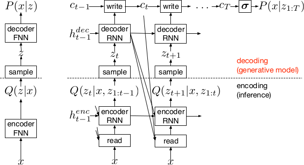
  * DRAW is a recurrent autoencoder for (primarily) images that uses attention mechanisms.
  * Like all autoencoders it has an encoder, a latent layer `Z` in the "middle" and a decoder.
  * Due to the recurrence, there are actually multiple autoencoders, one for each timestep (the number of timesteps is fixed).
  * DRAW has attention mechanisms which allow the model to decide where to look at in the input image ("glimpses") and where to write/draw to in the output image.
  * If the attention mechanisms are skipped, the model becomes a simple recurrent autoencoder.
  * By training the full autoencoder on a dataset and then only using the decoder, one can generate new images that look similar to the dataset images.


![DRAW Architecture](https://raw.githubusercontent.com/aleju/papers/master/neural-nets/images/DRAW_A_Recurrent_Neural_Network_for_Image_Generation__architecture.png?raw=true "DRAW Architecture")

*Basic recurrent architecture of DRAW.*


### How
  * General architecture
    * The encoder-decoder-pair follows the design of variational autoencoders.
    * The latent layer follows an n-dimensional gaussian distribution. The hyperparameters of that distribution (means, standard deviations) are derived from the output of the encoder using a linear transformation.
    * Using a gaussian distribution enables the use of the reparameterization trick, which can be useful for backpropagation.
    * The decoder receives a sample drawn from that gaussian distribution.
    * While the encoder reads from the input image, the decoder writes to an image canvas (where "write" is an addition, not a replacement of the old values).
    * The model works in a fixed number of timesteps. At each timestep the encoder performs a read operation and the decoder a write operation.
    * Both the encoder and the decoder receive the previous output of the encoder.
  * Loss functions
    * The loss function of the latent layer is the KL-divergence between that layer's gaussian distribution and a prior, summed over the timesteps.
    * The loss function of the decoder is the negative log likelihood of the image given the final canvas content under a bernoulli distribution.
    * The total loss, which is optimized, is the expectation of the sum of both losses (latent layer loss, decoder loss).
  * Attention
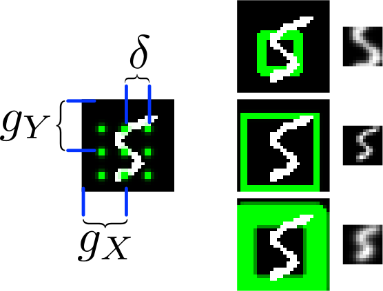
    * The selective read attention works on image patches of varying sizes. The result size is always NxN.
    * The mechanism has the following parameters:
        * `gx`: x-axis coordinate of the center of the patch
        * `gy`: y-axis coordinate of the center of the patch
        * `delta`: Strides. The higher the strides value, the larger the read image patch.
        * `sigma`: Standard deviation. The higher the sigma value, the more blurry the extracted patch will be.
        * `gamma`: Intensity-Multiplier. Will be used on the result.
        * All of these parameters are generated using a linear transformation applied to the decoder's output.
    * The mechanism places a grid of NxN gaussians on the image. The grid is centered at `(gx, gy)`. The gaussians are `delta` pixels apart from each other and have a standard deviation of `sigma`.
    * Each gaussian is applied to the image, the center pixel is read and added to the result.


![DRAW Attention](https://raw.githubusercontent.com/aleju/papers/master/neural-nets/images/DRAW_A_Recurrent_Neural_Network_for_Image_Generation__attention.png?raw=true "DRAW Attention")

*The basic attention mechanism. (gx, gy) is the read patch center. delta is the strides. On the right: Patches with different sizes/strides and standard deviations/blurriness.*


### Results
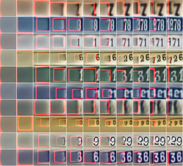
  * Realistic looking generated images for MNIST and SVHN.
  * Structurally OK, but overall blurry images for CIFAR-10.
  * Results with attention are usually significantly better than without attention.
  * Image generation without attention starts with a blurry image and progressively sharpens it.

![DRAW SVHN Results](https://raw.githubusercontent.com/aleju/papers/master/neural-nets/images/DRAW_A_Recurrent_Neural_Network_for_Image_Generation__svhn.png?raw=true "DRAW SVHN Results")

*Using DRAW with attention to generate new SVHN images.*

----------

### Rough chapter-wise notes

* 1. Introduction
  * The natural way to draw an image is in a step by step way (add some lines, then add some more, etc.).
  * Most generative neural networks however create the image in one step.
  * That removes the possibility of iterative self-correction, is hard to scale to large images and makes the image generation process dependent on a single latent distribution (input parameters).
  * The DRAW architecture generates images in multiple steps, allowing refinements/corrections.
  * DRAW is based on varational autoencoders: An encoder compresses images to codes and a decoder generates images from codes.
  * The loss function is a variational upper bound on the log-likelihood of the data.
  * DRAW uses recurrance to generate images step by step.
  * The recurrance is combined with attention via partial glimpses/foveations (i.e. the model sees only a small part of the image).
  * Attention is implemented in a differentiable way in DRAW.

* 2. The DRAW Network
  * The DRAW architecture is based on variational autoencoders:
    * Encoder: Compresses an image to latent codes, which represent the information contained in the image.
    * Decoder: Transforms the codes from the encoder to images (i.e. defines a distribution over images which is conditioned on the distribution of codes).
  * Differences to variational autoencoders:
    * Encoder and decoder are both recurrent neural networks.
    * The encoder receives the previous output of the decoder.
    * The decoder writes several times to the image array (instead of only once).
    * The encoder has an attention mechanism. It can make a decision about the read location in the input image.
    * The decoder has an attention mechanism. It can make a decision about the write location in the output image.
  * 2.1 Network architecture
    * They use LSTMs for the encoder and decoder.
    * The encoder generates a vector.
    * The decoder generates a vector.
    * The encoder receives at each time step the image and the output of the previous decoding step.
    * The hidden layer in between encoder and decoder is a distribution Q(Zt|ht^enc), which is a diagonal gaussian.
    * The mean and standard deviation of that gaussian is derived from the encoder's output vector with a linear transformation.
    * Using a gaussian instead of a bernoulli distribution enables the use of the reparameterization trick. That trick makes it straightforward to backpropagate "low variance stochastic gradients of the loss function through the latent distribution".
    * The decoder writes to an image canvas. At every timestep the vector generated by the decoder is added to that canvas.
  * 2.2 Loss function
    * The main loss function is the negative log probability: `-log D(x|ct)`, where `x` is the input image and `ct` is the final output image of the autoencoder. `D` is a bernoulli distribution if the image is binary (only 0s and 1s).
    * The model also uses a latent loss for the latent layer (between encoder and decoder). That is typical for VAEs. The loss is the KL-Divergence between Q(Zt|ht_enc) (`Zt` = latent layer, `ht_enc` = result of encoder) and a prior `P(Zt)`.
    * The full loss function is the expection value of both losses added up.
  * 2.3 Stochastic Data Generation
    * To generate images, samples can be picked from the latent layer based on a prior. These samples are then fed into the decoder. That is repeated for several timesteps until the image is finished.

* 3. Read and Write Operations
  * 3.1 Reading and writing without attention
    * Without attention, DRAW simply reads in the whole image and modifies the whole output image canvas at every timestep.
  * 3.2 Selective attention model
    * The model can decide which parts of the image to read, i.e. where to look at. These looks are called glimpses.
    * Each glimpse is defined by its center (x, y), its stride (zoom level), its gaussian variance (the higher the variance, the more blurry is the result) and a scalar multiplier (that scales the intensity of the glimpse result).
    * These parameters are calculated based on the decoder output using a linear transformation.
    * For an NxN patch/glimpse `N*N` gaussians are created and applied to the image. The center pixel of each gaussian is then used as the respective output pixel of the glimpse.
  * 3.3 Reading and writing with attention
    * Mostly the same technique from (3.2) is applied to both reading and writing.
    * The glimpse parameters are generated from the decoder output in both cases. The parameters can be different (i.e. read and write at different positions).
    * For RGB the same glimpses are applied to each channel.

* 4. Experimental results
  * They train on binary MNIST, cluttered MNIST, SVHN and CIFAR-10.
  * They then classfiy the images (cluttered MNIST) or generate new images (other datasets).
  * They say that these generated images are unique (to which degree?) and that they look realistic for MNIST and SVHN.
  * Results on CIFAR-10 are blurry.
  * They use binary crossentropy as the loss function for binary MNIST.
  * They use crossentropy as the loss function for SVHN and CIFAR-10 (color).
  * They used Adam as their optimizer.
  * 4.1 Cluttered MNIST classification
    * They classify images of cluttered MNIST. To do that, they use an LSTM that performs N read-glimpses and then classifies via a softmax layer.
    * Their model's error rate is significantly below a previous non-differentiable attention based model.
    * Performing more glimpses seems to decrease the error rate further.
  * 4.2 MNIST generation
    * They generate binary MNIST images using only the decoder.
    * DRAW without attention seems to perform similarly to previous models.
    * DRAW with attention seems to perform significantly better than previous models.
    * DRAW without attention progressively sharpens images.
    * DRAW with attention draws lines by tracing them.
  * 4.3 MNIST generation with two digits
    * They created a dataset of 60x60 images, each of them containing two random 28x28 MNIST images.
    * They then generated new images using only the decoder.
    * DRAW learned to do that.
    * Using attention, the model usually first drew one digit then the other.
  * 4.4 Street view house number generation
    * They generate SVHN images using only the decoder.
    * Results look quite realistic.
  * 4.5 Generating CIFAR images
    * They generate CIFAR-10 images using only the decoder.
    * Results follow roughly the structure of CIFAR-images, but look blurry.

http://blog.evjang.com/2016/06/understanding-and-implementing.html