This was a really cool-to-me paper that asked whether contrastive losses, of the kind that have found widespread success in semi-supervised domains, can add value in a supervised setting as well. In a semi-supervised context, contrastive loss works by pushing together the representations of an "anchor" data example with an augmented version of itself (which is taken as a positive or target, because the image is understood to not be substantively changed by being augmented), and pushing the representation of that example away from other examples in the batch, which are negatives in the sense that they are assumed to not be related to the anchor image. 

This paper investigates whether this same structure - of training representations of positives to be close relative to negatives - could be expanded to the supervised setting, where "positives" wouldn't just mean augmented versions of a single image, but augmented versions of other images belonging to the same class. This would ideally combine the advantages of self-supervised contrastive loss - that explicitly incentivizes invariance to augmentation-based changes - with the advantages of a supervised signal, which allows the representation to learn that it should also see instances of the same class as close to one another. 

https://i.imgur.com/pzKXEkQ.png

To evaluate the performance of this as a loss function, the authors first train the representation - either with their novel supervised contrastive loss SupCon, or with a control cross-entropy loss - and then train a linear regression with cross-entropy on top of that learned representation. (Just because, structurally, a contrastive loss doesn't lead to assigning probabilities to particular classes, even if it is supervised in the sense of capturing information relevant to classification in the representation) 

The authors investigate two versions of this contrastive loss, which differ, as shown below, in terms of the relative position of the sum and the log operation, and show that the L_out version dramatically outperforms (and I mean dramatically, with a top-one accuracy of 78.7 vs 67.4%). 

https://i.imgur.com/X5F1DDV.png

The authors suggest that the L_out version is superior in terms of training dynamics, and while I didn't fully follow their explanation, I believe it had to do with L_out version doing its normalization outside of the log, which meant it actually functioned as a multiplicative normalizer, as opposed to happening inside the log, where it would have just become an additive (or, really, subtractive) constant in the gradient term. Due to this stronger normalization, the authors positive the L_out loss was less noisy and more stable. 

Overall, the authors show that SupCon consistently (if not dramatically) outperforms cross-entropy when it comes to final accuracy. They also show that it is comparable in transfer performance to a self-supervised contrastive loss. One interesting extension to this work, which I'd enjoy seeing more explored in the future, is how the performance of this sort of loss scales with the number of different augmentations that performed of each element in the batch (this work uses two different augmentations, but there's no reason this number couldn't be higher, which would presumably give additional useful signal and robustness?)

Large-scale transformers on unsupervised text data have been wildly successful in recent years; arguably, the most successful single idea in the last ~3 years of machine learning. Given that, it's understandable that different domains within ML want to take their shot at seeing whether the same formula will work for them as well. This paper applies the principles of (1) transformers and (2) large-scale unlabeled data to the problem of learning informative embeddings of molecular graphs. 

Labeling is a problem in much of machine learning - it's costly, and narrowly defined in terms of a certain task - but that problem is even more exacerbated when it comes to labeling properties of molecules, since they typically require wetlab chemistry to empirically measure. Given that, and also given the fact that we often want to predict new properties - like effectiveness against a new targetable drug receptor - that we don't yet have data for, finding a way to learn and transfer from unsupervised data has the potential to be quite valuable in the molecular learning sphere. 

There are two main conceptual parts to this paper and its method - named GROVER, in true-to-ML-form tortured acronym style. The first is the actual architecture of their model itself, which combines both a message-passing Graph Neural Network to aggregate local information, and a Transformer to aggregate global information. The paper was a bit vague here, but the way I understand it is: 

https://i.imgur.com/JY4vRdd.png
- There are parallel GNN + Transformer stacks for both edges and nodes, each of which outputs both a node and edge embedding, for four embeddings total. I'll describe the one for nodes, and the parallel for edges operates the same way, except that hidden states live on edges rather than nodes, and attention is conducted over edges rather than nodes
- In the NodeTransformer version, a message passing NN (of I'm not sure how many layers) performs neighborhood aggregation (aggregating the hidden states of neighboring nodes and edges, then weight-transforming them, then aggregating again) until each node has a representation that has "absorbed" in information from a few hops out of its surrounding neighborhood. My understanding is that there is a separate MPNN for queries, keys, and values, and so each nodes end up with three different vectors for these three things.
- Multi-headed attention is then performed over these node representations, in the normal way, where all keys and queries are dot-product-ed together, and put into a softmax to calculate a weighted average over the values
- We now have node-level representations that combine both local and global information. These node representations are then aggregated into both node and edge representations, and each is put into a MLP layer and Layer Norm before finally outputting a node-based node and edge representation. This is then joined by an edge-based node and edge representation from the parallel stack. These are aggregated on a full-graph level to predict graph-level properties

https://i.imgur.com/NNl6v4Y.png

The other component of the GROVER model is the way this architecture is actually trained - without explicit supervised labels. The authors use two tasks - one local, and one global. The local task constructs labels based on local contextual properties of a given atom - for example, the atom here has one double-bonded Nitrogen and one single-bonded Oxygen in its local environment - and tries to predict those labels given the representations of that atom (or node). The global task uses RDKit (an analytically constructed molecular analysis kit) to identify 85 different modifs or functional groups in the molecule, and encodes those into an 85-long one-hot vector that is being predicted on a graph level. 

https://i.imgur.com/jzbYchA.png

With these two components, GROVER is pretrained on 10 million unlabeled molecules, and then evaluated in transfer settings where its representations are fine-tuned on small amounts of labeled data. The results are pretty impressive - it achieves new SOTA performance by relatively large amounts on all tasks, even relative to exist semi-supervised pretraining methods that similarly have access to more data. The authors perform ablations to show that it's important to do the graph-aggregation step before a transformer (the alternative being just doing a transformer on raw node and edge features), and also show that their architecture without pretraining (just used directly in downstream tasks) also performs worse. One thing I wish they'd directly ablated was the value-add of the local (also referred to as "contextual") and global semi-supervised tasks. Naively, I'd guess that most of the performance gain came from the global task, but it's hard to know without them having done the test directly.

The paper introduces nonnegative matrix factorization, a technique which used in fields such as chemometrics.  The problem formulation is this:

$$
\underset{W,H}{\text{argmin}} ~ d(X, WH) \\\\
\text{s.t.} ~W_{ij}, H_{ij} \ge 0
$$

Where:
- $X \in \mathbb{R}^{n \times m}$ is a matrix of data, for example, $n$ samples of $m$ features.  Each element of $X$ is nonnegative, as are the elements of $W$ and $H$.
- $W \in \mathbb{R}^{n \times k}$ represents how each of the $n$ samples belong to each of the $k$ "clusters".
- $H \in \mathbb{R}^{k \times m}$ describes each of the $k$ clusters in terms of the $m$ variables.
- $d$ is some cost function, for example, sum of squared differences.

The non-negativity constraint means the clusters (represented by the rows $W$ of $W$) describe clusters in terms of what features are present.  This may make interpretation easier in some instances, but makes the optimization problem more difficult.

The paper mentions two loss functions, sum of squared error:

$$
d(X,WH) = \sum_{ij} |X_{ij}-(WH)_{ij}|^2
$$

 and a measure similar to unnormalized Kullback-Leibler divergence:
 
 $$
d(X,WH) = \sum_{ij} \left( X_{ij} \log \frac{X_{ij}}{(WH)_{ij}} - X_{ij}+(WH)_{ij} \right)
$$

For each of these objectives, multiplicative update rules are given.  For squared error:

$$
H_{ij} \leftarrow H_{ij} \frac{(W^TX)_{ij}}{(W^TWH)}_{ij} ~~~
W_{ij} \leftarrow W_{ij} \frac{(XH^T)_{ij}}{(WHH^T)}_{ij}
$$

And for divergence:

$$
H_{ij} \leftarrow H_{ij} \frac{\sum_a W_{ai} X_{aj} / (WH)_{aj}} { \sum_b W_{bj}} ~~~~
W_{ij} \leftarrow W_{ij} \frac{\sum_a H_{ja} X_{ia} / (WH)_{ia}} { \sum_b H_{jb}}
$$

These rules are applied alternatingly; fix $W$ and update $H$, then fix $H$ and update $W$.

These multiplicative updates are essentially a diagonally rescaled gradient descent.  The authors then prove that these update rules do not increase the objective.  Future authors have pointed out that not increasing the cost does not imply convergence; e.g. the parameters could stop updating, without having reached a minima.  However, a trivial fix to the multiplicative update rules (ensuring no division by zero, by making 0 elements slightly positive) alleviates these problems.
  

If you read modern (that is, 2018-2020) papers using deep learning on molecular inputs, almost all of them use some variant of graph convolution. So, I decided to go back through the citation chain and read the earliest papers that thought to apply this technique to molecules, to get an idea of lineage of the technique within this domain. 

This 2015 paper, by Duvenaud et al, is the earliest one I can find. It focuses the entire paper on comparing differentiable, message-passing networks to the state of the art standard at the time, circular fingerprints (more on that in a bit). I really appreciated this approach, which, rather than trying to claim an unrealistic level of novelty, goes into detail on the prior approach, and carves out specific areas of difference. At a high level, the authors' claim is: our model is, in its simplest case, a more flexible and super version of existing work. The unspoken corollary, which ended up being proven true, is that the flexibility of the neural network structure makes it easy to go beyond this initial level of simplicity. 

Circular Fingerprinting (or, more properly, Extended-Connectivity Circular Fingerprints), is a fascinating algorithm that captures many of the elements of convolution: shared weights, a hierarchy of kernels that match patterns at different scales, and a clever way of aggregating information across an arbitrary number of input nodes. Mechanistically, Circular Fingerprints work by: 
1) Taking each atom, and creating a concatenated vector of its basic features, along with the basic features of each atom it's bonded to (with bonded neighbors quasi-randomly)

2) Calculating next-level features by applying some number of hash functions (roughly equivalent to convolutional kernels) to the neighborhood feature vector at the lower level to produce an integer 

3) For each feature, setting the value of the fingerprint vector to 1 at the index implied by the integer in step (2) 

4) Iterating this process at progressively higher layers, using the hash 

The effect of this is to assign each index of the vector to an binary feature (modulo hash collisions), where that feature is activated if an exact match is found to a structure within a given atom.  Its main downside is that (a) its "kernel" equivalents are fixed and not trainable, since they're just random hashes, and (b) its features represent *exact* matches to lower-level feature patterns, which means you can't have one feature activated to different degrees by variations on a pattern it's identifying.

https://i.imgur.com/V8FpfVE.png

Duvenaud et al present their alternative in terms of keeping a similar structure, but swapping out fixed and binary components for trainable (because differentiable) and continuous ones. Instead of concatenating a random sorting of atom neighbors to enforce invariance to sorting, they simply sum feature vectors across neighbors, which is also an order-invariantoperation. Instead of applying hash functions, they apply parametrized kernel functions, with the same parameters used across all aggregated neighborhood vectors . This will no longer look for exact matches, but will activate to the extent a structure within an atom matches against a kernel pattern. Then, these features are put into a softmax, which instead setting an index of a vector to a sharp one value, activates different feature indices in the final vector to differing degrees. The final fingerprint is simply the sum of these softmax feature activations for each atom. 

The authors do a few tests to confirm their substitution is working well, including starting out with a random network (to better approximate the random hash functions), comparing distances between atoms according to either the circular or neural footprint (which had a high correlation), and confirming that that performs similarly to circular fingerprints on a set of supervised learning tasks on modules. When they trained weights to be better than random on three such supervised tasks, they found that their model was comparable or better than circular fingerprints on all three (to break that down: it was basically equivalent on one, and notably better on the other two, according to mean squared error) 

This really is the simplest possible version of a message-passing or graph convolutional network (it doesn't use edge features, it doesn't calculate features of a neighbor-connection according to the features of each node, etc), but it's really satisfying to see it laid out as a next-step alternative that offered value just by stepping away from exact-match feature dynamics and non-random functions, even without all the sophisticated additions that would later be added to such models.

  * They suggest a variation of Faster R-CNN.
  * Their network detects bounding boxes (e.g. of people, cars) in images *and also* segments the objects within these bounding boxes (i.e. classifies for each pixel whether it is part of the object or background).
  * The model runs roughly at the same speed as Faster R-CNN.

### How
  * The architecture and training is mostly the same as in Faster R-CNN:
    * Input is an image.
    * The *backbone* network transforms the input image into feature maps. It consists of convolutions, e.g. initialized with ResNet's weights.
    * The *RPN* (Region Proposal Network) takes the feature maps and classifies for each location whether there is a bounding box at that point (with some other stuff to regress height/width and offsets).
      This leads to a large number of bounding box candidates (region proposals) per image.
    * *RoIAlign*: Each region proposal's "area" is extracted from the feature maps and converted into a fixed-size `7x7xF` feature map (with F input filters). (See below.)
    * The *head* uses the region proposal's features to perform
      * Classification: "is the bounding box of a person/car/.../background"
      * Regression: "bounding box should have width/height/offset so and so"
      * Segmentation: "pixels so and so are part of this object's mask"
    * Rough visualization of the architecture:
      * ![Architecture](https://raw.githubusercontent.com/aleju/papers/master/neural-nets/images/Mask_R-CNN/architecture.jpg?raw=true "Architecture")
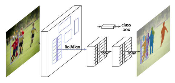
  * RoIAlign
    * This is very similar to RoIPooling in Faster R-CNN.
    * For each RoI, RoIPooling first "finds" the features in the feature maps that lie within the RoI's rectangle. Then it max-pools them to create a fixed size vector.
    * Problem: The coordinates where an RoI starts and ends may be non-integers. E.g. the top left corner might have coordinates `(x=2.5, y=4.7)`.
      RoIPooling simply rounds these values to the nearest integers (e.g. `(x=2, y=5)`).
      But that can create pooled RoIs that are significantly off, as the feature maps with which RoIPooling works have high (total) stride (e.g. 32 pixels in standard ResNets).
      So being just one cell off can easily lead to being 32 pixels off on the input image.
    * For classification, being some pixels off is usually not that bad. For masks however it can significantly worsen the results, as these have to be pixel-accurate.
    * In RoIAlign this is compensated by not rounding the coordinates and instead using bilinear interpolation to interpolate between the feature map's cells.
    * Each RoI is pooled by RoIAlign to a fixed sized feature map of size `(H, W, F)`, with H and W usually being 7 or 14. (It can also generate different sizes, e.g. `7x7xF` for classification and more accurate `14x14xF` for masks.)
    * If H and W are `7`, this leads to `49` cells within each plane of the pooled feature maps.
    * Each cell again is a rectangle -- similar to the RoIs -- and pooled with bilinear interpolation.
      More exactly, each cell is split up into four sub-cells (top left, top right, bottom right, bottom left).
      Each of these sub-cells is pooled via bilinear interpolation, leading to four values per cell.
      The final cell value is then computed using either an average or a maximum over the four sub-values.
  * Segmentation
    * They add an additional branch to the *head* that gets pooled RoI as inputs and processes them seperately from the classification and regression (no connections between the branches).
    * That branch does segmentation. It is fully convolutional, similar to many segmentation networks.
    * The result is one mask per class.
    * There is no softmax per pixel over the classes, as classification is done by a different branch.
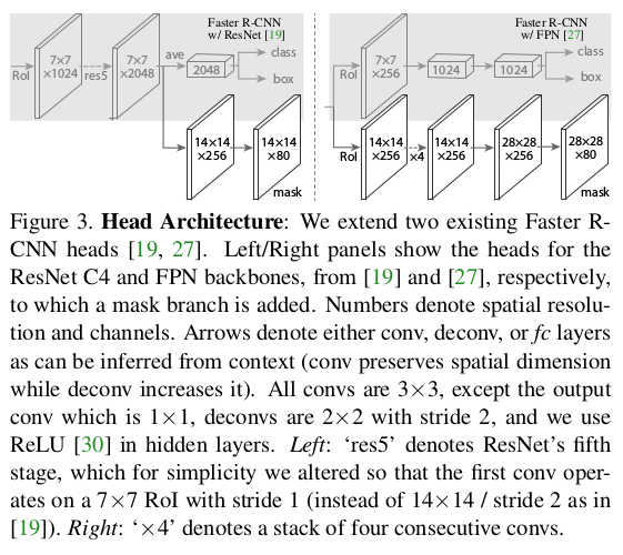
  * Base networks
    * Their *backbone* networks are either ResNet or ResNeXt (in the 50 or 102 layer variations).
    * Their *head* is either the fourth/fifth module from ResNet/ResNeXt (called *C4* (fourth) or *C5* (fifth)) or they use the second half from the FPN network (called *FPN*).
    * They denote their networks via `backbone-head`, i.e. ResNet-101-FPN means that their backbone is ResNet-101 and their head is FPN.
    * Visualization of the different heads:
      * ![Architecture heads](https://raw.githubusercontent.com/aleju/papers/master/neural-nets/images/Mask_R-CNN/head.jpg?raw=true "Architecture heads")
  * Training
    * Training happens in basically the same way as Faster R-CNN.
    * They just add an additional loss term to the total loss (`L = L_classification + L_regression + L_mask`). `L_mask` is based on binary cross-entropy.
    * For each predicted RoI, the correct mask is the intersection between that RoI's area and the correct mask.
    * They only train masks for RoIs that are positive (overlap with ground truth bounding boxes).
    * They train for 120k iterations at learning rate 0.02 and 40k at 0.002 with weight decay 0.0002 and momentum 0.9.
  * Test
    * For the *C4*-head they sample up to 300 region proposals from the RPN (those with highest confidence values). For the FPN head they sample up to 1000, as FPN is faster.
    * They sample masks only for the 100 proposals with highest confidence values.
    * Each mask is turned into a binary mask using a threshold of 0.5.

### Results
  * Instance Segmentation
    * They train and test on COCO.
    * They can outperform the best competitor by a decent margin (AP 37.1 vs 33.6 for FCIS+++ with OHEM).
    * Their model especially performs much better when there is overlap between bounding boxes.
    * Ranking of their models: ResNeXt-101-FPN > ResNet-101-FPN > ResNet-50-FPN > ResNet-101-C4 > ResNet-50-C4.
    * Using sigmoid instead of softmax (over classes) for the mask prediction significantly improves results by 5.5 to 7.1 points AP (depending on measurement method).
    * Predicting only one mask per RoI (class-agnostic) instead of C masks (where C is the number of classes) only has a small negative effect on AP (about 0.6 points).
    * Using RoIAlign instead of RoIPooling has significant positive effects on the AP of around 5 to 10 points (if a network with C5 head is chosen, which has a high stride of 32). Effects are smaller for small strides and FPN head.
    * Using fully convolutional networks for the mask branch performs better than fully connected layers (1-3 points AP).
    * Examples results on COCO vs FCIS (note the better handling of overlap):
      * ![Examples COCO](https://raw.githubusercontent.com/aleju/papers/master/neural-nets/images/Mask_R-CNN/examples_overlap.jpg?raw=true "Examples COCO")
  * Bounding-Box-Detection
    * Training additionally on masks seems to improve AP for bounding boxes by around 1 point (benefit from multi-task learning).
  * Timing
    * Around 200ms for ResNet-101-FPN. (M40 GPU)
    * Around 400ms for ResNet-101-C4.
  * Human Pose Estimation
    * The mask branch can be used to predict keypoint (landmark) locations on human bodies (i.e. locations of hands, feet etc.).
    * This is done by using one mask per keypoint, initializing it to `0` and setting the keypoint location to `1`.
    * By doing this, Mask R-CNN can predict keypoints roughly as good as the current leading models (on COCO), while running at 5fps.
  * Cityscapes
    * They test their model on the cityscapes dataset.
    * They beat previous models with significant margins. This is largely due to their better handling of overlapping instances.
    * They get their best scores using a model that was pre-trained on COCO.
    * Examples results on cityscapes:
      * ![Examples Cityscapes](https://raw.githubusercontent.com/aleju/papers/master/neural-nets/images/Mask_R-CNN/examples_cityscapes.jpg?raw=true "Examples Cityscapes")