* Deep plain/ordinary networks usually perform better than shallow networks.
  * However, when they get too deep their performance on the *training* set decreases. That should never happen and is a shortcoming of current optimizers.
  * If the "good" insights of the early layers could be transferred through the network unaltered, while changing/improving the "bad" insights, that effect might disappear.

###  What residual architectures are
  * Residual architectures use identity functions to transfer results from previous layers unaltered.
  * They change these previous results based on results from convolutional layers.
  * So while a plain network might do something like `output = convolution(image)`, a residual network will do `output = image + convolution(image)`.
  * If the convolution resorts to just doing nothing, that will make the result a lot worse in the plain network, but not alter it at all in the residual network.
  * So in the residual network, the convolution can focus fully on learning what positive changes it has to perform, while in the plain network it *first* has to learn the identity function and then what positive changes it can perform.

### How it works
  * Residual architectures can be implemented in most frameworks. You only need something like a split layer and an element-wise addition.
  * Use one branch with an identity function and one with 2 or more convolutions (1 is also possible, but seems to perform poorly). Merge them with the element-wise addition.
  * Rough example block (for a 64x32x32 input):
https://i.imgur.com/NJVb9hj.png  
  * An example block when you have to change the dimensionality (e.g. here from 64x32x32 to 128x32x32):
https://i.imgur.com/9NXvTjI.png
  * The authors seem to prefer using either two 3x3 convolutions or the chain of 1x1 then 3x3 then 1x1. They use the latter one for their very deep networks.
  * The authors also tested:
    * To use 1x1 convolutions instead of identity functions everywhere. Performed a bit better than using 1x1 only for dimensionality changes. However, also computation and memory demands.
    * To use zero-padding for dimensionality changes (no 1x1 convs, just fill the additional dimensions with zeros). Performed only a bit worse than 1x1 convs and a lot better than plain network architectures.
  * Pooling can be used as in plain networks. No special architectures are necessary.
  * Batch normalization can be used as usually (before nonlinearities).

### Results
  * Residual networks seem to perform generally better than similarly sized plain networks.
  * They seem to be able to achieve similar results with less computation.
  * They enable well-trainable very deep architectures with up to 1000 layers and more.
  * The activations of the residual layers are low compared to plain networks. That indicates that the residual networks indeed only learn to make "good" changes and default to "if in doubt, change nothing".


![Building blocks](https://raw.githubusercontent.com/aleju/papers/master/neural-nets/images/Deep_Residual_Learning_for_Image_Recognition__building_blocks.png?raw=true "Building blocks")

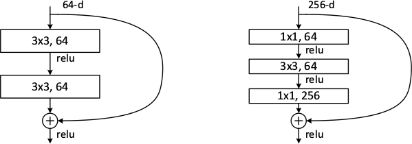
*Examples of basic building blocks (other architectures are possible). The paper doesn't discuss the placement of the ReLU (after add instead of after the layer).*


![Activations](https://raw.githubusercontent.com/aleju/papers/master/neural-nets/images/Deep_Residual_Learning_for_Image_Recognition__activations.png?raw=true "Activations")

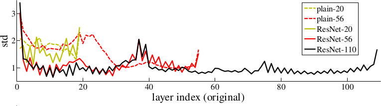
*Activations of layers (after batch normalization, before nonlinearity) throughout the network for plain and residual nets. Residual networks have on average lower activations.*

-------------------------

### Rough chapter-wise notes

* (1) Introduction
  * In classical architectures, adding more layers can cause the network to perform worse on the training set.
  * That shouldn't be the case. (E.g. a shallower could be trained and then get a few layers of identity functions on top of it to create a deep network.)
  * To combat that problem, they stack residual layers.
  * A residual layer is an identity function and can learn to add something on top of that.
  * So if `x` is an input image and `f(x)` is a convolution, they do something like `x + f(x)` or even `x + f(f(x))`.
  * The classical architecture would be more like `f(f(f(f(x))))`.
  * Residual architectures can be easily implemented in existing frameworks using skip connections with identity functions (split + merge).
  * Residual architecture outperformed other in ILSVRC 2015 and COCO 2015.

* (3) Deep Residual Learning
  * If some layers have to fit a function `H(x)` then they should also be able to fit `H(x) - x` (change between `x` and `H(x)`).
  * The latter case might be easier to learn than the former one.
  * The basic structure of a residual block is `y = x + F(x, W)`, where `x` is the input image, `y` is the output image (`x + change`) and `F(x, W)` is the residual subnetwork that estimates a good change of `x` (W are the subnetwork's weights).
  * `x` and `F(x, W)` are added using element-wise addition.
  * `x` and the output of `F(x, W)` must be have equal dimensions (channels, height, width).
  * If different dimensions are required (mainly change in number of channels) a linear projection `V` is applied to `x`: `y = F(x, W) + Vx`. They use a 1x1 convolution for `V` (without nonlinearity?).
  * `F(x, W)` subnetworks can contain any number of layer. They suggest 2+ convolutions. Using only 1 layer seems to be useless.
  * They run some tests on a network with 34 layers and compare to a 34 layer network without residual blocks and with VGG (19 layers).
  * They say that their architecture requires only 18% of the FLOPs of VGG. (Though a lot of that probably comes from VGG's 2x4096 fully connected layers? They don't use any fully connected layers, only convolutions.)
  * A critical part is the change in dimensionality (e.g. from 64 kernels to 128). They test (A) adding the new dimensions empty (padding), (B) using the mentioned linear projection with 1x1 convolutions and (C) using the same linear projection, but on all residual blocks (not only for dimensionality changes).
  * (A) doesn't add parameters, (B) does (i.e. breaks the pattern of using identity functions).
  * They use batch normalization before each nonlinearity.
  * Optimizer is SGD.
  * They don't use dropout.

* (4) Experiments
  * When testing on ImageNet an 18 layer plain (i.e. not residual) network has lower training set error than a deep 34 layer plain network.
  * They argue that this effect does probably not come from vanishing gradients, because they (a) checked the gradient norms and they looked healthy and (b) use batch normaliaztion.
  * They guess that deep plain networks might have exponentially low convergence rates.
  * For the residual architectures its the other way round. Stacking more layers improves the results.
  * The residual networks also perform better (in error %) than plain networks with the same number of parameters and layers. (Both for training and validation set.)
  * Regarding the previously mentioned handling of dimensionality changes:
    * (A) Pad new dimensions: Performs worst. (Still far better than plain network though.)
    * (B) Linear projections for dimensionality changes: Performs better than A.
    * (C) Linear projections for all residual blocks: Performs better than B. (Authors think that's due to introducing new parameters.)
  * They also test on very deep residual networks with 50 to 152 layers.
  * For these deep networks their residual block has the form `1x1 conv -> 3x3 conv -> 1x1 conv` (i.e. dimensionality reduction, convolution, dimensionality increase).
  * These deeper networks perform significantly better.
  * In further tests on CIFAR-10 they can observe that the activations of the convolutions in residual networks are lower than in plain networks.
  * So the residual networks default to doing nothing and only change (activate) when something needs to be changed.
  * They test a network with 1202 layers. It is still easily optimizable, but overfits the training set.
  * They also test on COCO and get significantly better results than a Faster-R-CNN+VGG implementation.

Liu et al. propose fine-pruning, a combination of weight pruning and fine-tuning to defend against backdoor attacks on neural networks. Specifically, they consider a setting where training is outsourced to a machine learning service; the attacker has access to the network and training set, however, any change in network architecture would be easily detected. Thus, the attacker tries to inject backdoors through data poisening. As defense against such attacks, the authors propose to identify and prune weights that are not used for the actual tasks but only for the backdoor inputs.  This defense can then be combined with fine-tuning and, as shown in experiments, is able to make backdoor attacks less effective – even when considering an attacker aware of this defense.

Also find this summary at [davidstutz.de](https://davidstutz.de/category/reading/).

TLDR; The authors train a word-level NMT where UNK tokens in both source and target sentence are replaced by character-level RNNs that produce word representations. The authors can thus train a fast word-based system that still generalized that doesn't produce unknown words. The best system achieves a new state of the art BLEU score of 19.9 in WMT'15 English to Czech translation.


#### Key Points

- Source Sentence: Final hidden state of character-RNN is used as word representation.
- Source Sentence: Character RNNs always initialized with 0 state to allow efficient pre-training 
- Target: Produce word-level sentence including UNK first and then run the char-RNNs
- Target: Two ways to initialize char-RNN: With same hidden state as word-RNN (same-path), or with its own representation (separate-path)
- Authors find that attention mechanism is critical for pure character-based NMT models


#### Notes

- Given that the authors demonstrate the potential of character-based models, is the hybrid approach the right direction? If we had more compute power, would pure character-based models win?

## Keywords
Triplet-loss , face embedding , harmonic embedding

---
## Summary

### Introduction

**Goal of the paper**    
A unified system is given for face verification , recognition and clustering.
Use of a 128 float  pose and illumination invariant feature vector or embedding in the euclidean space.
* Face Verification : Same faces of the person gives feature vectors that have a very close L2 distance between them. 
* Face recognition : Face recognition becomes a clustering task in the embedding space
	
**Previous work**    
* Previous use of deep learning made use of an bottleneck layer to represent face as an embedding of  1000s  dimension  vector.
* Some other techniques use PCA to reduce the dimensionality of the embedding for comparison.

**Method**
* This method makes use of inception style CNN to get an embedding of each face.
* The thumbnails of the face image are the tight crop of the face area with only scaling and translation done on them.
	
**Triplet Loss**
Triplet loss  makes use of two matching face thumbnails and a non-matching thumbnail. The loss function tries to reduce the distance between the matching pair while increasing the separation between the the non-matching pair of images.

**Triplet Selection**
* Selection of triplets is done such that samples are hard-positive or hard-negative .
* Hardest negative can lead to local minima early in the training and a collapse model in a few cases
* Use of semi-hard negatives help to improve the convergence speed while at the same time reach nearer to the global minimum.

**Deep Convolutional Network**
* Training is done using SGD (Stochastic gradient descent) with Backpropagation and AdaGrad
* The training is done on two networks :
    - Zeiler&Fergus architecture with model depth of 22 and 140 million parameters
    - GoogLeNet style inception model with 6.6 to 7.5 million parameters.

**Experiment**
* Study of the following cases are done :
    - Quality of the jpeg image : The validation rate of model improves with the JPEG quality upto a certain threshold.

    - Embedding dimensionality : The dimension of the embedding increases from 64 to 128,256 and then gradually starts to decrease at 512 dimensions. 

    - No. of images in the training data set 



**Results classification accuracy** :
   - LFW(Labelled faces in the wild) dataset : 98.87% 0.15
   - Youtube Faces DB : 95.12%  .39
On clustering tasks the model was able to work on a wide varieties of face images and is invariant to pose , lighting and also age.

**Conclusion**

* The model can be extended further to improve the overall accuracy.
* Training networks to run on smaller systems like mobile phones.
* There is need for improving the training efficiency.

---

## Notes 

* Harmonic embedding is a set of embedding that we get from different models but are compatible to each other. This helps to improve future upgrades and transitions to a newer model

* To make the embeddings compatible with different models , harmonic-triplet loss and the generated triplets must be compatible with each other

## Open research questions

* Better understanding of the error cases.
* Making the model more compact for embedded and mobile use cases.
* Methods to reduce the training times.

  * They define four subtasks of image understanding:
    * *Classification*: Assign a single label to a whole image.
    * *Captioning*: Assign a sequence of words (description) to a whole image*
    * *Detection*: Find objects/regions in an image and assign a single label to each one.
    * *Dense Captioning*: Find objects/regions in an image and assign a sequence of words (description) to each one.
  * DenseCap accomplishes the fourth task, i.e. it is a model that finds objects/regions in images and describes them with natural language.

### How
  * Their model consists of four subcomponents, which run for each image in sequence:
    * (1) **Convolutional Network**:
      * Basically just VGG-16.
    * (2) **Localization Layer**:
      * This layer uses a convolutional network that has mostly the same architecture as in the "Faster R-CNN" paper.
      * That ConvNet is applied to a grid of anchor points on the image.
      * For each anchor point, it extracts the features generated by the VGG-Net (model 1) around that point.
      * It then generates the attributes of `k` (default: 12) boxes using a shallow convolutional net. These attributes are (roughly): Height, width, center x, center y, confidence score.
      * It then extracts the features of these boxes from the VGG-Net output (model 1) and uses bilinear sampling to project them onto a fixed size (height, width) for the next model. The result are the final region proposals.
      * By default every image pixel is an anchor point, which results in a large number of regions. Hence, subsampling is used during training and testing.
    * (3) **Recognition Network**:
      * Takes a region (flattened to 1d vector) and projects it onto a vector of length 4096.
      * It uses fully connected layers to do that (ReLU, dropout).
      * Additionally, the network takes the 4096 vector and outputs new values for the region's position and confidence (for late fine tuning).
      * The 4096 vectors of all regions are combined to a matrix that is fed into the next component (RNN).
      * The intended sense of the this component seems to be to convert the "visual" features of each region to a more abstract, high-dimensional representation/description.
    * (4) **RNN Language Model**:
      * The take each 4096 vector and apply a fully connected layer + ReLU to it.
      * Then they feed it into an LSTM, followed by a START token.
      * The LSTM then generates word (as one hot vectors), which are fed back into the model for the next time step.
      * This is continued until the LSTM generates an END token.
  * Their full loss function has five components:
    * Binary logistic loss for the confidence values generated by the localization layer.
    * Binary logistic loss for the confidence values generated by the recognition layer.
    * Smooth L1 loss for the region dimensions generated by the localization layer.
    * Smooth L1 loss for the region dimensiosn generated by the recognition layer.
    * Cross-entropy at every time-step of the language model.
  * The whole model can be trained end-to-end.

* Results
  * They mostly use the Visual Genome dataset.
  * Their model finds lots of good regions in images.
  * Their model generates good captions for each region. (Only short captions with simple language however.)
  * The model seems to love colors. Like 30-50% of all captions contain a color. (Probably caused by the dataset?)
  * They compare to EdgeBoxes (other method to find regions in images). Their model seems to perform better.
  * Their model requires about 240ms per image (test time).
  * The generated regions and captions enable one to search for specific objects in images using text queries.


![Architecture](https://raw.githubusercontent.com/aleju/papers/master/neural-nets/images/DenseCap__architecture.png?raw=true "Architecture.")

*Architecture of the whole model. It starts with the VGG-Net ("CNN"), followed by the localization layer, which generates region proposals. Then the recognition network converts the regions to abstract high-dimensional representations. Then the language model ("RNN") generates the caption.*


![Elephant image with dense captioning.](https://raw.githubusercontent.com/aleju/papers/master/neural-nets/images/DenseCap__elephant.png?raw=true "Elephant image with dense captioning.")

![Airplane image with dense captioning.](https://raw.githubusercontent.com/aleju/papers/master/neural-nets/images/DenseCap__airplane.png?raw=true "Airplane image with dense captioning.")


--------------------

### Rough chapter-wise notes

* (1) Introduction
  * They define four subtasks of visual scene understanding:
    * Classification: Assign a single label to a whole image
    * Captioning: Assign a sequence of words (description) to a whole image
    * Detection: Find objects in an image and assign a single label to each one
    * Dense Captioning: Find objects in an image and assign a sequence of words (description) to each one
  * They developed a model for dense captioning.
  * It has two three important components:
    * A convoltional network for scene understanding
    * A localization layer for region level predictions. It predicts regions of interest and then uses bilinear sampling to extract the activations of these regions.
    * A recurrent network as the language model
  * They evaluate the model on the large-scale Visual Genome dataset (94k images, 4.1M region captions).

* (3) Model
  * Model architecture
    * Convolutional Network
      * They use VGG-16, but remove the last pooling layer.
      * For an image of size W, H the output is 512xW/16xH/16.
      * That output is the input into the localization layer.
    * Fully Convolutional Localization Layer
      * Input to this layer: Activations from the convolutional network.
      * Output of this layer: Regions of interest, as fixed-sized representations.
        * For B Regions:
          * Coordinates of the bounding boxes (matrix of shape Bx4)
          * Confidence scores (vector of length B)
          * Features (matrix of shape BxCxXxY)
      * Method: Faster R-CNN (pooling replaced by bilinear interpolation)
      * This layer is fully differentiable.
      * The localization layer predicts boxes at anchor points.
      * At each anchor point it proposes `k` boxes using a small convolutional network. It assigns a confidence score and coordinates (center x, center y, height, width) to each proposal.
      * For an image with size 720x540 and k=12 the model would have to predict 17,280 boxes, hence subsampling is used.
      * During training they use minibatches with 256/2 positive and 256/2 negative region examples. A box counts as a positive example for a specific image if it has high overlap (intersection) with an annotated box for that image.
      * During test time they use greedy non-maximum suppression (NMS) (?) to subsample the 300 most confident boxes.
      * The region proposals have varying box sizes, but the output of the localization layer (which will be fed into the RNN) is ought to have fixed sizes.
      * So they project each proposed region onto a fixed sized region. They use bilinear sampling for that projection, which is differentiable.
    * Recognition network
      * Each region is flattened to a one-dimensional vector.
      * That vector is fed through 2 fully connected layers (unknown size, ReLU, dropout), ending with a 4096 neuron layer.
      * The confidence score and box coordinates are also adjusted by the network during that process (fine tuning).
    * RNN Language Model
      * Each region is translated to a sentence.
      * The region is fed into an LSTM (after a linear layer + ReLU), followed by a special START token.
      * The LSTM outputs multiple words as one-hot-vectors, where each vector has the length `V+1` (i.e. vocabulary size + END token).
      * Loss function is average crossentropy between output words and target words.
      * During test time, words are sampled until an END tag is generated.
  * Loss function
    * Their full loss function has five components:
      * Binary logistic loss for the confidence values generated by the localization layer.
      * Binary logistic loss for the confidence values generated by the recognition layer.
      * Smooth L1 loss for the region dimensions generated by the localization layer.
      * Smooth L1 loss for the region dimensiosn generated by the recognition layer.
      * Cross-entropy at every time-step of the language model.
    * The language model term has a weight of 1.0, all other components have a weight of 0.1.
  * Training an optimization
    * Initialization: CNN pretrained on ImageNet, all other weights from `N(0, 0.01)`.
    * SGD for the CNN (lr=?, momentum=0.9)
    * Adam everywhere else (lr=1e-6, beta1=0.9, beta2=0.99)
    * CNN is trained after epoch 1. CNN's first four layers are not trained.
    * Batch size is 1.
    * Image size is 720 on the longest side.
    * They use Torch.
    * 3 days of training time.

* (4) Experiments
  * They use the Visual Genome Dataset (94k images, 4.1M regions with captions)
  * Their total vocabulary size is 10,497 words. (Rare words in captions were replaced with `<UNK>`.)
  * They throw away annotations with too many words as well as images with too few/too many regions.
  * They merge heavily overlapping regions to single regions with multiple captions.
  * Dense Captioning
    * Dense captioning task: The model receives one image and produces a set of regions, each having a caption and a confidence score.
    * Evaluation metrics
      * Evaluation of the output is non-trivial.
      * They compare predicted regions with regions from the annotation that have high overlap (above a threshold).
      * They then compare the predicted caption with the captions having similar METEOR score (above a threshold).
      * Instead of setting one threshold for each comparison they use multiple thresholds. Then they calculate the Mean Average Precision using the various pairs of thresholds.
    * Baseline models
      * Sources of region proposals during test time:
        * GT: Ground truth boxes (i.e. found by humans).
        * EB: EdgeBox (completely separate and pretrained system).
        * RPN: Their localization and recognition networks trained separately on VG regions dataset (i.e. trained without the RNN language model).
      * Models:
        * Region RNN model: Apparently the recognition layer and the RNN language model, trained on predefined regions. (Where do these regions come from? VG training dataset?)
        * Full Image RNN model: Apparently the recognition layer and the RNN language model, trained on full images from MSCOCO instead of small regions.
        * FCLN on EB: Apparently the recognition layer and the RNN language model, trained on regions generated by EdgeBox (EB) (on VG dataset?).
        * FCLN: Apparently their full model (trained on VG dataset?).
    * Discrepancy between region and image level statistics
      * When evaluating the models only on METEOR (language "quality"), the *Region RNN model* consistently outperforms the *Full Image RNN model*.
      * That's probably because the *Full Image RNN model* was trained on captions of whole images, while the *Region RNN model* was trained on captions of small regions, which tend to be a bit different from full image captions.
    * RPN outperforms external region proposals
      * Generating region proposals via RPN basically always beats EB.
    * Our model outperforms individual region description
      * Their full jointly trained model (FCLN) achieves the best results.
      * The full jointly trained model performs significantly better than `RPN + Region RNN model` (i.e. separately trained region proposal and region captioning networks).
    * Qualitative results
      * Finds plenty of good regions and generates reasonable captions for them.
      * Sometimes finds the same region twice.
    * Runtime evaluation
      * 240ms on 720x600 image with 300 region proposals.
      * 166ms on 720x600 image with 100 region proposals.
      * Recognition of region proposals takes up most time.
      * Generating region proposals takes up the 2nd most time.
      * Generating captions for regions (RNN) takes almost no time.
  * Image Retrieval using Regions and Captions
    * They try to search for regions based on search queries.
    * They search by letting their FCLN network or EB generate 100 region proposals per network. Then they calculate per region the probability of generating the search query as the caption. They use that probability to rank the results.
    * They pick images from the VG dataset, then pick captions within those images as search query. Then they evaluate the ranking of those images for the respective search query.
    * The results show that the model can learn to rank objects, object parts, people and actions as expected/desired.
    * The method described can also be used to detect an arbitrary number of distinct classes in images (as opposed to the usual 10 to 1000 classes), because the classes are contained in the generated captions.