This paper directly relies on understanding [Gumbel-Softmax][gs] ([Concrete][]) sampling.

The place to start thinking about this paper is in terms of a distribution over possible permutations. You could, for example, have a categorical distribution over all the permutation matrices of a given size. Of size 2 this is easy:

```
p(M)   0.1    0.9

M:     1, 0   0, 1
       0, 1   1, 0
```

You could apply the Gumbel-Softmax trick to this, and other selections of permutation matrices in small dimensions, but the number of possible permutations grows factorially with the dimension. If you want to infer the order of $100$ items, you now have a categorical over $100!$ variables, and you can't even store that number in floating point.

By breaking up and applying a normalised weight to each permutation matrix, we are effectively doing a [Naive Birkhoff-Von Neumann decomposition][naive] to return a sample from the space of Doubly Stochastic matrices. This paper proposes *much* more efficient ways to sample from this space in a way that is amenable to stochastic variational (read *SGD*) methods, such that they have an experiment working with permutations of 278 variables.

There are two ingredients to a good stochastic variational recipe:

1. A differentiable sampling method; for example (most famously): $x = \mu + \sigma \epsilon \text{ where } \epsilon \sim \mathcal{N}(0,1)$
2. A density over this sampling distribution; in the preceding example: $\mathcal{N}(\mu, \sigma)$

This paper presents two recipes: Stick-breaking transformations and Rounding towards permutation matrices.

Stick-breaking
--------------------

[Shakir Mohamed wrote a good blog post on stick-breaking methods.][sticks]

One problem, which you could guess from the categorical-over-permutations example above, is we can't possibly store a probability for each permutation matrix ($N!$ is a lot of numbers to store). Stick-breaking gives us another way to represent these probabilities implicitly through $B \in [0,1]^{(N-1)\times (N-1)}$. The row `x` gets recursively broken up like this:

```
    B_11    B_12*(1-x[:1].sum())     1-x[:2].sum()
x: |-------|------------------------|---------------------|
    x[0]    x[1]                     x[2]
    <---------------------------------------------------->
                               1.0
```

For two dimensions, this becomes a little more complicated (and is actually a novel part of this paper) so I'll just refer you to the paper and say: *this is also possible in two dimensions*.

OK, so now to sample from the distribution of Doubly Stochastic matrices, you just need to sample $(N-1) \times (N-1)$ values in the range $[0,1]$. The authors sample a Gaussian and pass it through a sigmoid. Along with a temperature parameter, the values get pushed closer to 0 or 1 and the result is a permutation matrix.

To get the density, the authors *appear to* (this would probably be annoying in high dimensions) automatically differentiate through the $N^2$ steps of the stick-breaking transformation to get the Jacobian and use change of variables.

Rounding
-------------

This method is more idiosyncratic, so I'll just copy the steps straight from the paper:

> 1. Input $Z \in R^{N \times N} $, $M \in R_+^{N \times N}$, and $V \in  R_+^{N \times N}$;
> 2. Map $M \to \tilde{M}$, a point in the Birkhoff polytope, using the [Sinkhorn-Knopp algorithm][sk];
> 3. Set $\Psi = \tilde{M} + V \odot Z$ where $\odot$ denotes elementwise multiplication;
> 4. Find $\text{round}(\Psi)$, the nearest permutation matrix to $\Psi$, using the [Hungarian algorithm][ha];
> 5. Output $X = \tau \Psi + (1- \tau)\text{round}(\Psi)$.

So you can just schedule $\tau \to 0$ and you'll be moving your distribution to be a distribution over permutation matrices.

The big problem with this is we *can't easily get the density*. Step 4 is not differentiable. However, the authors argue the function is still piecewise-linear so we can just get around this. Once they've done that, it's possible to evaluate the density by change of variables again.

Results
----------

On a synthetic permutation matching problem, the rounding method gets a better match to the true posterior (the synthetic problem is small enough to enumerate the true posterior). It also performs better than competing methods on a real matching problem; matching the activations in neurons of C. Elegans to the location of neurons in the known connectome.

[sticks]: http://blog.shakirm.com/2015/12/machine-learning-trick-of-the-day-6-tricks-with-sticks/
[naive]: https://en.wikipedia.org/wiki/Doubly_stochastic_matrix#Birkhoff_polytope_and_Birkhoff.E2.80.93von_Neumann_theorem
[gs]: http://www.shortscience.org/paper?bibtexKey=journals/corr/JangGP16
[concrete]: http://www.shortscience.org/paper?bibtexKey=journals/corr/1611.00712
[sk]: https://en.wikipedia.org/wiki/Sinkhorn%27s_theorem#Sinkhorn-Knopp_algorithm
[ha]: https://en.wikipedia.org/wiki/Hungarian_algorithm

The propagation rule used in this paper is the following:

$$
H^l = \sigma \left(\tilde{D}^{-\frac{1}{2}} \tilde{A} \tilde{D}^{-\frac{1}{2}} H^{l-1} W^l \right)
$$

Where $\tilde{A}$ is the [adjacency matrix][adj] of the undirected graph (with self connections, so has a diagonal of 1s and is symmetric) and $H^l$ are the hidden activations at layer $l$. The $D$ matrices are performing row normalisation, $\tilde{D}^{-\frac{1}{2}} \tilde{A} \tilde{D}^{-\frac{1}{2}}$ is [equivalent to][pygcn] (with $\tilde{A}$ as `mx`):

```
rowsum = np.array(mx.sum(1))            # sum along rows
r_inv = np.power(rowsum, -1).flatten()  # 1./rowsum elementwise
r_mat_inv = sp.diags(r_inv)             # cast to sparse diagonal matrix
mx = r_mat_inv.dot(mx)                  # sparse matrix multiply
```

The symmetric way to express this is part of the [symmetric normalized Laplacian][laplace]. This work, and the [other][hammond] [work][defferrard] on graph convolutional networks, is motivated by convolving a parametric filter over $x$. Convolution becomes easy if we can perform a *graph Fourier transform* (don't worry I don't understand this either), but that requires us having access to eigenvectors of the normalized graph Laplacian (which is expensive).

[Hammond's early paper][hammond] suggested getting around this problem by using Chebyshev polynomials for the approximation. This paper takes the approximation even further, using only *first order* Chebyshev polynomial, on the assumption that this will be fine because the modeling capacity can be picked up by the deep neural network.

That's how the propagation rule above is derived, but we don't really need to remember the details. In practice $\tilde{D}^{-\frac{1}{2}} \tilde{A} \tilde{D}^{-\frac{1}{2}} = \hat{A}$ is calculated prior and using a graph convolutional network involves multiplying your activations by this sparse matrix at every hidden layer. If you're thinking in terms of a batch with $N$ examples and $D$ features, this multiplication happens *over the examples*, mixing datapoints together (according to the graph structure). If you want to think of this in an orthodox deep learning way, it's the following:

```
activations = F.linear(H_lm1, W_l)         # (N,D)
activations = activations.permute(1,0)     # (D,N)
activations = F.linear(activations, hat_A) # (D,N)
activations = activations.permute(1,0)     # (N,D)
H_l = F.relu(activations)
```

**Won't this be really slow though, $\hat{A}$ is $(N,N)$!** Yes, if you implemented it that way it would be very slow. But, many deep learning frameworks support sparse matrix operations ([although maybe not the backward pass][sparse]). Using that, a graph convolutional layer can be implemented [quite easily][pygcnlayer].

**Wait a second, these are batches, not minibatches?** Yup, minibatches are future work.

**What are the experimental results, though?** There are experiments showing this works well for semi-supervised experiments on graphs, as advertised. Also, the many approximations to get the propagation rule at the top are justified by experiment.

**This summary is bad.** Fine, smarter people have written their own posts: [the author's][kipf], [Ferenc's][ferenc].

[adj]: https://en.wikipedia.org/wiki/Adjacency_matrix
[pygcn]: https://github.com/tkipf/pygcn/blob/master/pygcn/utils.py#L56-L63
[laplace]: https://en.wikipedia.org/wiki/Laplacian_matrix#Symmetric_normalized_Laplacian
[hammond]: https://arxiv.org/abs/0912.3848
[defferrard]: https://arxiv.org/abs/1606.09375
[sparse]: https://discuss.pytorch.org/t/does-pytorch-support-autograd-on-sparse-matrix/6156/7
[pygcnlayer]: https://github.com/tkipf/pygcn/blob/master/pygcn/layers.py#L35-L68
[kipf]: https://tkipf.github.io/graph-convolutional-networks/
[ferenc]: http://www.inference.vc/how-powerful-are-graph-convolutions-review-of-kipf-welling-2016-2/

#### Goal:
+ Diagnostic and drug code prediction on a subsequent visit using diagnostic codes, medications, procedures and date of previous visits.
+ Predict when the next visit to the doctor will happen.

#### Dataset:

+ Sutter Health Palo Alto Medical Foundation - primary care - case-control study for heart failure.

![Dataset](https://raw.githubusercontent.com/tiagotvv/ml-papers/master/clinical-data/images/Choi2016_dataset.png?raw=true "Dataset information")

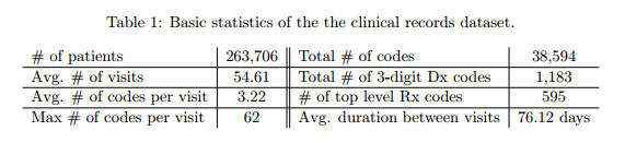
+ Patients with fewer than two visits were excluded.
+ Inputs:
  + ICD-9 codes,
  + GPI drug codes
  + codes for CPT procedures
+ Records are time-stamped with the patient's visiting time.
+ If a patient receives multiple codes on the same visit, they all receive the same timestamp.
+ Granularity of codes - group subcategories:
  + ICD-9 3 digits: 1183 unique codes
  + GPI Drug class: 595 single groups
+ Target: y = [diagnosis, drug] - vector of 1183 + 595 = 1778 dimensions.

#### Architecture:
+ Gated Recurrent Units (GRU)

![GRU architecture](https://raw.githubusercontent.com/tiagotvv/ml-papers/master/clinical-data/images/Choi2016_gru.png?raw=true "Gated Recurrent Unit (GRU)")


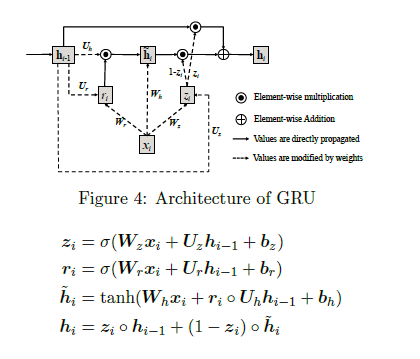+ The input vector x is one-hot encoded and has a dimension of 40000. The first layer tries to reduce dimensionality.
+ Two approaches to dimensionality reduction (embedding matrix W_emb)
  + W_emb is learned together with the model.
  + W_emb is pre-trained using techniques such as word2vec.
+ Loss function: cross entropy for codes + quadratic error for forecasting visits.
+ Prediction layer codes: Softmax / Prediction layer of the next time visit: ReLu.

#### Experiments and Results:

+ Code available on GitHub: https://github.com/mp2893/doctorai
+ Implementation in Theano - Training with 2 Nvidia Tesla K80 GPUs

*Methodology*:
+ Dataset split: 85% training, 15% test.
+ RNN trained for 20 epochs.
+ L2 regularization for both the vector of coefficients of the codes and for the vector of coefficients of the next visit (lambda = 0.001) - Dropout between GRU and prediction layer (and between GRU layers if there are more than 1).
+ 2000 neurons in the hidden layer

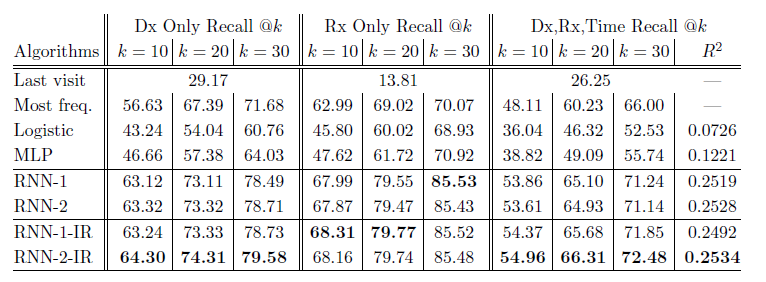
*Baselines*:

+ Frequency: The codes from the previous visit are repeated on the new visit. Good baseline for the case of patients whose condition tends to stabilize over time.
+ Top k most frequent codes from the previous visit.
+ Logistic Regression and Multilayer Perceptron. Uses the last 5 visits to predict the next.



*Metrics*:

+ top-k recall emulates the behavior of physicians when making a differential diagnosis

    top-k recall = # of true positives in the top k predictions / number of true positives

+ R^2 used to evaluate the performance of the next visit prediction.
  + Predict logarithm of time duration between visits to reduce the impact of very long intervals.

*Results Table*:

  + RNN-1: RNN with a single hidden layer initialized with a random orthogonal matrix for W_emb.
  + RNN-2: RNN with two hidden layers initialized with a random orthogonal matrix for W_emb.
  + RNN-1-IR: RNN using a single hidden layer initialized embedding matrix w emb with the Skip-gram vectors trained on the entire dataset. 
  + RNN-2-IR: RNN with two hidden layers initialized embedding matrix W_emb with the Skip-gram vectors trained on the entire dataset.    

![Results](https://raw.githubusercontent.com/tiagotvv/ml-papers/master/clinical-data/images/Choi2016_results1.png?raw=true "Forecasting future medical activities")


+ Performance varies according to the number of patient visits:
  + Networks learn best when they observe more records.
  + Patients with frequent visits are sicker patients. In a way, it is easier to predict the future in these cases.

![Number of visits](https://raw.githubusercontent.com/tiagotvv/ml-papers/master/clinical-data/images/Choi2016_results2.png?raw=true "Doctor AI performance as it knows more about the patient")


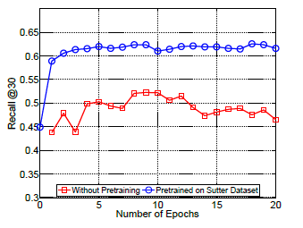
+ Performance of Doctor AI in other datasets:
  + Potential to transfer knowledge accross hospitals. Pre-train Doctor AI on Sutter Health dataset and fine-tuned in MIMIC II dataset.
  
![Transfer knowledge](https://raw.githubusercontent.com/tiagotvv/ml-papers/master/clinical-data/images/Choi2016_results3.png?raw=true "Performance of Doctor AI in other datasets")

#### Extras
+ There is an interview about the paper at the [Data Skeptic](https://dataskeptic.com/blog/episodes/2017/doctor-ai) podcast.

1. U-NET learns segmentation in an end to end images.
2. They solved Challenges are
        * Very few annotated images (approx. 30 per application).
        * Touching objects of the same class.
# How:
* Input image is fed in to the network, then the data is propagated through the network along all possible path at the end segmentation maps comes out.
* In U-net architecture, each blue box corresponds to a multi-channel feature map. The number of channels is denoted on top of the box. The x-y-size is provided at the lower left edge of the box. White boxes represent copied feature maps. The arrows denote the different operations.
https://i.imgur.com/Usxmv6r.png
* In two 3x3 convolutions (unpadded convolutions), each followed by a rectified linear unit (ReLU) and a 2x2 max pooling operation with stride 2for down sampling. At each down sampling step they double the number of feature channels.
* Contracting path (left side from up to down) is increases the feature channel and reduces the steps and an expansive path (right side from down to up) consists of sequence of up convolution and concatenation with the corresponds high resolution features from contracting path.
* The network does not have any fully connected layers and only uses the valid part of each convolution, i.e., the segmentation map only contains the pixels, for which the full context is available in the input image.

## Challenges:
1. Overlap-tile strategy for seamless segmentation of arbitrary large images:
     * To predict the pixels in the border region of the image, the missing context is extrapolated by mirroring the input image.
     * In fig, segmentation of the yellow area uses input data of the blue area and the raw data extrapolation by mirroring.
https://i.imgur.com/NUbBRUG.png
2. Augment training data using deformation:
    * They use excessive data augmentation by applying elastic deformations to the available training images. 
    * Then the network to learn invariance to such deformations, without the need to see these transformations in the annotated image corpus.
    * Deformation used to be the most common variation in tissue and realistic deformations can be simulated efficiently. 
https://i.imgur.com/CyC8Hmd.png
3. Segmentation of touching object of the same class:
    * They propose the use of a weighted loss, where the separating background labels between touching cells obtain a large weight in the loss function.
    * Ensure separation of touching objects, in that segmentation mask for training (inserted background between touching objects) get the loss weights for each pixel.
https://i.imgur.com/ds7psDB.png
4. Segmentation of neural structure in electro-microscopy(EM):
    * Ongoing challenge since ISBI 2012 in this dataset structures with low contrast, fuzzy membranes and other cell components.
    * The training data is a set of 30 images (512x512 pixels) from serial section transmission electron microscopy of the Drosophila first instar larva ventral nerve cord (VNC). Each image comes with corresponding fully annotated ground truth segmentation map for cells(white) and membranes (black).
    * An evaluation can be obtained by sending the predicted membrane probability map to the organizers. The evaluation is done by thresholding  the map at 10 different levels and computation of the warping error, the Rand error and the pixel error.

### Results:
* The u-net (averaged over 7 rotated versions of the input data) achieves with-out any further pre or post-processing a warping error of 0.0003529, a rand-error of 0.0382 and a pixel error of 0.0611.
https://i.imgur.com/6BDrByI.png
* ISBI cell tracking challenge 2015, one of the dataset contains cell phase contrast microscopy has strong shape variations,weak outer borders, strong irrelevant inner borders and cytoplasm has same structure like background.
https://i.imgur.com/vDflYEH.png
* The first data set PHC-U373 contains Glioblastoma-astrocytoma U373 cells on a polyacrylimide substrate recorded by phase contrast microscopy- It contains 35 partially annotated training images. Here we achieve an average IOU ("intersection over union") of 92%,which is significantly better than the second best algorithm with 83%.
https://i.imgur.com/of4rAYP.png
* The second data set DIC-HeLa are HeLa cells on a flat glass recorded by differential interference contrast (DIC) microscopy - It contains 20 partially annotated training images. Here we achieve an average IOU of 77.5% which is significantly better than the second best algorithm with 46%.
https://i.imgur.com/Y9wY6Lc.png

# Object detection system overview.

https://i.imgur.com/vd2YUy3.png
 
1.	takes an input image,
2.	extracts around 2000 bottom-up region proposals, 
3.	computes features for each proposal using a large convolutional neural network (CNN), and then
4.	classifies each region using class-specific linear SVMs.
* R-CNN achieves a mean average precision (mAP) of 53.7% on PASCAL VOC 2010.
* On the 200-class ILSVRC2013 detection dataset, R-CNN’s mAP is 31.4%, a large improvement over OverFeat , which had the previous best result at 24.3%.

## There is a 2 challenges faced in object detection 
1.	localization problem
2.	labeling the data

1 localization problem :
*  One approach frames localization as a regression problem.  they report a mAP of 30.5% on VOC 2007 compared to the 58.5% achieved by our method.
* An alternative is to build a sliding-window detector.  considered adopting a sliding-window approach increases the number of convolutional layers to 5, have very large receptive fields (195 x 195 pixels) and strides (32x32 pixels) in the input image, which makes precise localization within the sliding-window paradigm.

2 labeling the data:
* The conventional solution to this problem is to use unsupervised pre-training, followed by supervise fine-tuning 
* supervised pre-training on a large auxiliary dataset (ILSVRC), followed by domain specific fine-tuning on a small dataset (PASCAL),
* fine-tuning for detection improves mAP performance by 8 percentage points. 
* Stochastic gradient descent via back propagation was used to  effective for training convolutional neural networks (CNNs)
 
##  Object detection with R-CNN
This  system consists of three modules
* The first generates category-independent region proposals. These proposals define the set of candidate detections available to our detector.
*  The second module is a large convolutional neural network that extracts a fixed-length feature vector from each region.
* The third module is a set of class specific linear SVMs.

Module design

1 Region proposals 
* which detect mitotic cells by applying a CNN to regularly-spaced square crops.
* use selective search method in fast mode (Capture All Scales, Diversification, Fast to Compute).
* the time spent computing region proposals and features (13s/image on a GPU or 53s/image on a CPU)

2 Feature extraction.
* extract a 4096-dimensional feature vector from each region proposal using the Caffe  implementation of the CNN 
* Features are computed by forward propagating a mean-subtracted 227x227 RGB image through five convolutional layers and two fully connected layers.
* warp all pixels in a tight bounding box around it to the required size
* The feature matrix is typically 2000x4096 

3 Test time detection
* At test time, run selective search on the test image to extract around 2000 region proposals (we use selective search’s “fast mode” in all experiments).
*  warp each proposal and forward propagate it through the CNN in order to compute features. Then, for each class, we score each extracted feature vector using the SVM trained for that class.
* Given all scored regions in an image, we apply a greedy non-maximum suppression (for each class independently) that rejects a region if it has an intersection-over union (IoU) overlap with a higher scoring selected region larger than a learned threshold.
## Training

1 Supervised pre-training:
 * pre-trained the CNN on a large auxiliary dataset (ILSVRC2012 classification)  using image-level annotations only (bounding box labels are not available for this data)

2  Domain-specific fine-tuning.
* use the stochastic gradient descent (SGD) training of the CNN parameters using only warped region proposals with  learning rate of 0.001.

3  Object category classifiers.
*   use intersection-over union (IoU) overlap threshold method  to label a region with The overlap threshold of 0.3.
* Once features are extracted and training labels are applied, we optimize one linear SVM per class.
* adopt the standard hard negative mining method to fit large training data in memory.

### Results on PASCAL VOC 201012

1  VOC 2010
* compared against four strong baselines including SegDPM, DPM, UVA, Regionlets. 
* Achieve a large improvement in mAP, from 35.1% to 53.7% mAP,  while also being much faster
 https://i.imgur.com/0dGX9b7.png
2 ILSVRC2013 detection.
* ran R-CNN on the 200-class ILSVRC2013 detection dataset
* R-CNN achieves a mAP of 31.4%
https://i.imgur.com/GFbULx3.png
#### Performance layer-by-layer, without fine-tuning
1 pool5 layer 
* which is the max pooled output of the network’s fifth and final convolutional layer.
*The pool5 feature map is 6 x6 x 256 = 9216 dimensional
* each pool5 unit has a receptive field of 195x195 pixels in the original 227x227 pixel input

2 Layer fc6
* fully connected to pool5
*  it multiplies a 4096x9216 weight matrix by the pool5 feature map (reshaped as a 9216-dimensional vector) and then adds a vector of biases

3 Layer fc7
* It is implemented by multiplying the features computed by fc6 by a 4096 x 4096 weight matrix, and similarly adding a vector of biases and applying half-wave rectification
#### Performance layer-by-layer, with fine-tuning
* CNN’s parameters  fine-tuned on PASCAL.
* fine-tuning increases mAP by 8.0 % points to 54.2%

### Network architectures
* 16-layer deep network, consisting of 13 layers of 3 _ 3 convolution kernels, with five max pooling layers interspersed, and topped with three fully-connected layers. We refer to this network as “O-Net” for OxfordNet and the baseline as “T-Net” for TorontoNet.
* RCNN with O-Net substantially outperforms R-CNN with TNet, increasing mAP from 58.5% to 66.0%
* drawback in terms of compute time, with in terms of compute time, with than T-Net.

1 The ILSVRC2013 detection dataset
* dataset is split into three sets: train (395,918), val (20,121), and test (40,152) 

#### CNN features for segmentation.
* full R-CNN: The first strategy (full) ignores the re region’s shape and computes CNN features directly on the warped window. Two regions might have very similar bounding boxes while having very little overlap. 
* fg R-CNN: the second strategy (fg) computes CNN features only on a region’s foreground mask. We replace the background with the mean input so that background regions are zero after mean subtraction.
* full+fg R-CNN: The third strategy (full+fg) simply concatenates the full and fg features
 https://i.imgur.com/n1bhmKo.png