* DRAW = deep recurrent attentive writer
  * DRAW is a recurrent autoencoder for (primarily) images that uses attention mechanisms.
  * Like all autoencoders it has an encoder, a latent layer `Z` in the "middle" and a decoder.
  * Due to the recurrence, there are actually multiple autoencoders, one for each timestep (the number of timesteps is fixed).
  * DRAW has attention mechanisms which allow the model to decide where to look at in the input image ("glimpses") and where to write/draw to in the output image.
  * If the attention mechanisms are skipped, the model becomes a simple recurrent autoencoder.
  * By training the full autoencoder on a dataset and then only using the decoder, one can generate new images that look similar to the dataset images.


![DRAW Architecture](https://raw.githubusercontent.com/aleju/papers/master/neural-nets/images/DRAW_A_Recurrent_Neural_Network_for_Image_Generation__architecture.png?raw=true "DRAW Architecture")

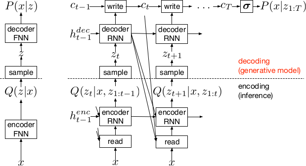
*Basic recurrent architecture of DRAW.*


### How
  * General architecture
    * The encoder-decoder-pair follows the design of variational autoencoders.
    * The latent layer follows an n-dimensional gaussian distribution. The hyperparameters of that distribution (means, standard deviations) are derived from the output of the encoder using a linear transformation.
    * Using a gaussian distribution enables the use of the reparameterization trick, which can be useful for backpropagation.
    * The decoder receives a sample drawn from that gaussian distribution.
    * While the encoder reads from the input image, the decoder writes to an image canvas (where "write" is an addition, not a replacement of the old values).
    * The model works in a fixed number of timesteps. At each timestep the encoder performs a read operation and the decoder a write operation.
    * Both the encoder and the decoder receive the previous output of the encoder.
  * Loss functions
    * The loss function of the latent layer is the KL-divergence between that layer's gaussian distribution and a prior, summed over the timesteps.
    * The loss function of the decoder is the negative log likelihood of the image given the final canvas content under a bernoulli distribution.
    * The total loss, which is optimized, is the expectation of the sum of both losses (latent layer loss, decoder loss).
  * Attention
    * The selective read attention works on image patches of varying sizes. The result size is always NxN.
    * The mechanism has the following parameters:
        * `gx`: x-axis coordinate of the center of the patch
        * `gy`: y-axis coordinate of the center of the patch
        * `delta`: Strides. The higher the strides value, the larger the read image patch.
        * `sigma`: Standard deviation. The higher the sigma value, the more blurry the extracted patch will be.
        * `gamma`: Intensity-Multiplier. Will be used on the result.
        * All of these parameters are generated using a linear transformation applied to the decoder's output.
    * The mechanism places a grid of NxN gaussians on the image. The grid is centered at `(gx, gy)`. The gaussians are `delta` pixels apart from each other and have a standard deviation of `sigma`.
    * Each gaussian is applied to the image, the center pixel is read and added to the result.


![DRAW Attention](https://raw.githubusercontent.com/aleju/papers/master/neural-nets/images/DRAW_A_Recurrent_Neural_Network_for_Image_Generation__attention.png?raw=true "DRAW Attention")

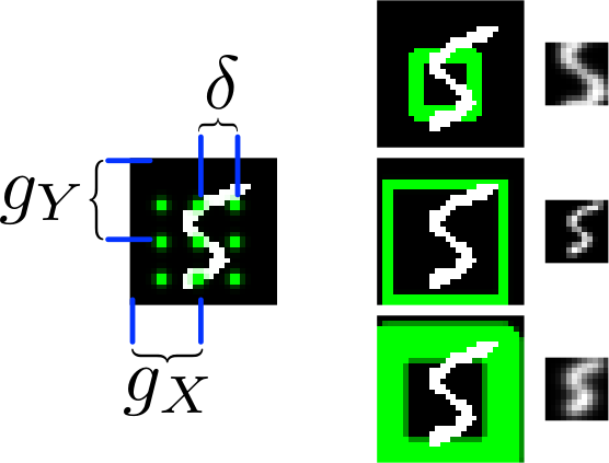
*The basic attention mechanism. (gx, gy) is the read patch center. delta is the strides. On the right: Patches with different sizes/strides and standard deviations/blurriness.*


### Results
  * Realistic looking generated images for MNIST and SVHN.
  * Structurally OK, but overall blurry images for CIFAR-10.
  * Results with attention are usually significantly better than without attention.
  * Image generation without attention starts with a blurry image and progressively sharpens it.

![DRAW SVHN Results](https://raw.githubusercontent.com/aleju/papers/master/neural-nets/images/DRAW_A_Recurrent_Neural_Network_for_Image_Generation__svhn.png?raw=true "DRAW SVHN Results")

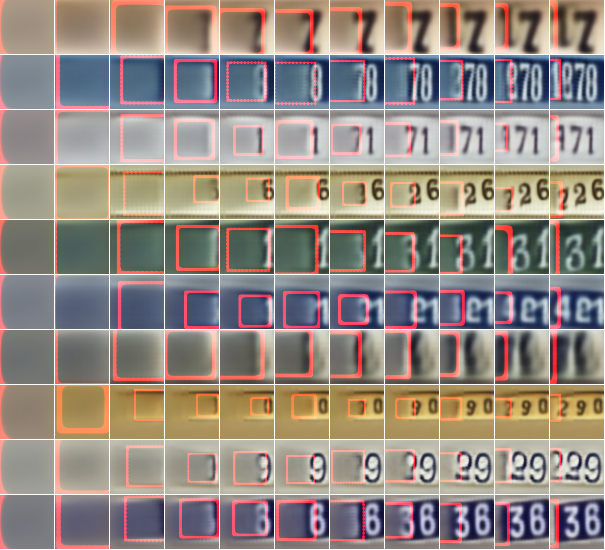
*Using DRAW with attention to generate new SVHN images.*

----------

### Rough chapter-wise notes

* 1. Introduction
  * The natural way to draw an image is in a step by step way (add some lines, then add some more, etc.).
  * Most generative neural networks however create the image in one step.
  * That removes the possibility of iterative self-correction, is hard to scale to large images and makes the image generation process dependent on a single latent distribution (input parameters).
  * The DRAW architecture generates images in multiple steps, allowing refinements/corrections.
  * DRAW is based on varational autoencoders: An encoder compresses images to codes and a decoder generates images from codes.
  * The loss function is a variational upper bound on the log-likelihood of the data.
  * DRAW uses recurrance to generate images step by step.
  * The recurrance is combined with attention via partial glimpses/foveations (i.e. the model sees only a small part of the image).
  * Attention is implemented in a differentiable way in DRAW.

* 2. The DRAW Network
  * The DRAW architecture is based on variational autoencoders:
    * Encoder: Compresses an image to latent codes, which represent the information contained in the image.
    * Decoder: Transforms the codes from the encoder to images (i.e. defines a distribution over images which is conditioned on the distribution of codes).
  * Differences to variational autoencoders:
    * Encoder and decoder are both recurrent neural networks.
    * The encoder receives the previous output of the decoder.
    * The decoder writes several times to the image array (instead of only once).
    * The encoder has an attention mechanism. It can make a decision about the read location in the input image.
    * The decoder has an attention mechanism. It can make a decision about the write location in the output image.
  * 2.1 Network architecture
    * They use LSTMs for the encoder and decoder.
    * The encoder generates a vector.
    * The decoder generates a vector.
    * The encoder receives at each time step the image and the output of the previous decoding step.
    * The hidden layer in between encoder and decoder is a distribution Q(Zt|ht^enc), which is a diagonal gaussian.
    * The mean and standard deviation of that gaussian is derived from the encoder's output vector with a linear transformation.
    * Using a gaussian instead of a bernoulli distribution enables the use of the reparameterization trick. That trick makes it straightforward to backpropagate "low variance stochastic gradients of the loss function through the latent distribution".
    * The decoder writes to an image canvas. At every timestep the vector generated by the decoder is added to that canvas.
  * 2.2 Loss function
    * The main loss function is the negative log probability: `-log D(x|ct)`, where `x` is the input image and `ct` is the final output image of the autoencoder. `D` is a bernoulli distribution if the image is binary (only 0s and 1s).
    * The model also uses a latent loss for the latent layer (between encoder and decoder). That is typical for VAEs. The loss is the KL-Divergence between Q(Zt|ht_enc) (`Zt` = latent layer, `ht_enc` = result of encoder) and a prior `P(Zt)`.
    * The full loss function is the expection value of both losses added up.
  * 2.3 Stochastic Data Generation
    * To generate images, samples can be picked from the latent layer based on a prior. These samples are then fed into the decoder. That is repeated for several timesteps until the image is finished.

* 3. Read and Write Operations
  * 3.1 Reading and writing without attention
    * Without attention, DRAW simply reads in the whole image and modifies the whole output image canvas at every timestep.
  * 3.2 Selective attention model
    * The model can decide which parts of the image to read, i.e. where to look at. These looks are called glimpses.
    * Each glimpse is defined by its center (x, y), its stride (zoom level), its gaussian variance (the higher the variance, the more blurry is the result) and a scalar multiplier (that scales the intensity of the glimpse result).
    * These parameters are calculated based on the decoder output using a linear transformation.
    * For an NxN patch/glimpse `N*N` gaussians are created and applied to the image. The center pixel of each gaussian is then used as the respective output pixel of the glimpse.
  * 3.3 Reading and writing with attention
    * Mostly the same technique from (3.2) is applied to both reading and writing.
    * The glimpse parameters are generated from the decoder output in both cases. The parameters can be different (i.e. read and write at different positions).
    * For RGB the same glimpses are applied to each channel.

* 4. Experimental results
  * They train on binary MNIST, cluttered MNIST, SVHN and CIFAR-10.
  * They then classfiy the images (cluttered MNIST) or generate new images (other datasets).
  * They say that these generated images are unique (to which degree?) and that they look realistic for MNIST and SVHN.
  * Results on CIFAR-10 are blurry.
  * They use binary crossentropy as the loss function for binary MNIST.
  * They use crossentropy as the loss function for SVHN and CIFAR-10 (color).
  * They used Adam as their optimizer.
  * 4.1 Cluttered MNIST classification
    * They classify images of cluttered MNIST. To do that, they use an LSTM that performs N read-glimpses and then classifies via a softmax layer.
    * Their model's error rate is significantly below a previous non-differentiable attention based model.
    * Performing more glimpses seems to decrease the error rate further.
  * 4.2 MNIST generation
    * They generate binary MNIST images using only the decoder.
    * DRAW without attention seems to perform similarly to previous models.
    * DRAW with attention seems to perform significantly better than previous models.
    * DRAW without attention progressively sharpens images.
    * DRAW with attention draws lines by tracing them.
  * 4.3 MNIST generation with two digits
    * They created a dataset of 60x60 images, each of them containing two random 28x28 MNIST images.
    * They then generated new images using only the decoder.
    * DRAW learned to do that.
    * Using attention, the model usually first drew one digit then the other.
  * 4.4 Street view house number generation
    * They generate SVHN images using only the decoder.
    * Results look quite realistic.
  * 4.5 Generating CIFAR images
    * They generate CIFAR-10 images using only the decoder.
    * Results follow roughly the structure of CIFAR-images, but look blurry.

  * The authors define in this paper a special loss function (DeePSiM), mostly for autoencoders.
  * Usually one would use a MSE of euclidean distance as the loss function for an autoencoder. But that loss function basically always leads to blurry reconstructed images.
  * They add two new ingredients to the loss function, which results in significantly sharper looking images.

### How
  * Their loss function has three components:
    * Euclidean distance in image space (i.e. pixel distance between reconstructed image and original image, as usually used in autoencoders)
    * Euclidean distance in feature space. Another pretrained neural net (e.g. VGG, AlexNet, ...) is used to extract features from the original and the reconstructed image. Then the euclidean distance between both vectors is measured.
    * Adversarial loss, as usually used in GANs (generative adversarial networks). The autoencoder is here treated as the GAN-Generator. Then a second network, the GAN-Discriminator is introduced. They are trained in the typical GAN-fashion. The loss component for DeePSiM is the loss of the Discriminator. I.e. when reconstructing an image, the autoencoder would learn to reconstruct it in a way that lets the Discriminator believe that the image is real.
  * Using the loss in feature space alone would not be enough as that tends to lead to overpronounced high frequency components in the image (i.e. too strong edges, corners, other artefacts).
  * To decrease these high frequency components, a "natural image prior" is usually used. Other papers define some function by hand. This paper uses the adversarial loss for that (i.e. learns a good prior).
  * Instead of training a full autoencoder (encoder + decoder) it is also possible to only train a decoder and feed features - e.g. extracted via AlexNet - into the decoder.

### Results
  * Using the DeePSiM loss with a normal autoencoder results in sharp reconstructed images.
  * Using the DeePSiM loss with a VAE to generate ILSVRC-2012 images results in sharp images, which are locally sound, but globally don't make sense. Simple euclidean distance loss results in blurry images.
  * Using the DeePSiM loss when feeding only image space features (extracted via AlexNet) into the decoder leads to high quality reconstructions. Features from early layers will lead to more exact reconstructions.
  * One can again feed extracted features into the network, but then take the reconstructed image, extract features of that image and feed them back into the network. When using DeePSiM, even after several iterations of that process the images still remain semantically similar, while their exact appearance changes (e.g. a dog's fur color might change, counts of visible objects change).

![Generated images](https://raw.githubusercontent.com/aleju/papers/master/neural-nets/images/Generating_Images_with_Perceptual_Similarity_Metrics_based_on_Deep_Networks__generated_images.png?raw=true "Generated images")

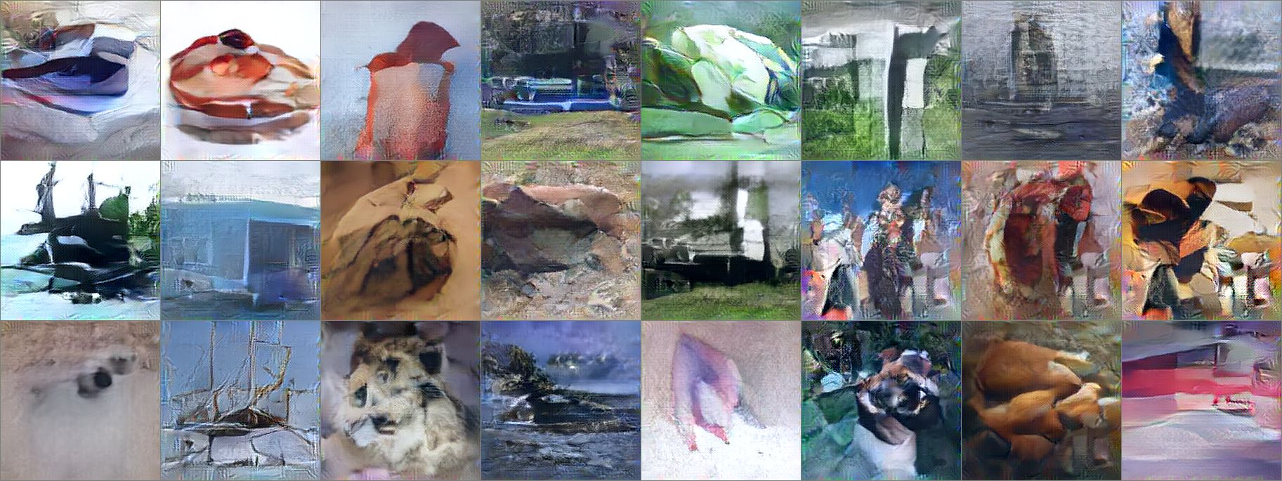
*Images generated with a VAE using DeePSiM loss.*


![Reconstructed images](https://raw.githubusercontent.com/aleju/papers/master/neural-nets/images/Generating_Images_with_Perceptual_Similarity_Metrics_based_on_Deep_Networks__reconstructed.png?raw=true "Reconstructed images")

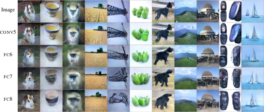
*Images reconstructed from features fed into the network. Different AlexNet layers (conv5 - fc8) were used to generate the features. Earlier layers allow more exact reconstruction.*


![Iterated reconstruction](https://raw.githubusercontent.com/aleju/papers/master/neural-nets/images/Generating_Images_with_Perceptual_Similarity_Metrics_based_on_Deep_Networks__reconstructed_multi.png?raw=true "Iterated reconstruction")

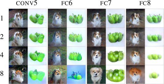
*First, images are reconstructed from features (AlexNet, layers conv5 - fc8 as columns). Then, features of the reconstructed images are fed back into the network. That is repeated up to 8 times (rows). Images stay semantically similar, but their appearance changes.*

--------------------

### Rough chapter-wise notes

* (1) Introduction
  * Using a MSE of euclidean distances for image generation (e.g. autoencoders) often results in blurry images.
  * They suggest a better loss function that cares about the existence of features, but not as much about their exact translation, rotation or other local statistics.
  * Their loss function is based on distances in suitable feature spaces.
  * They use ConvNets to generate those feature spaces, as these networks are sensitive towards important changes (e.g. edges) and insensitive towards unimportant changes (e.g. translation).
  * However, naively using the ConvNet features does not yield good results, because the networks tend to project very different images onto the same feature vectors (i.e. they are contractive). That leads to artefacts in the generated images.
  * Instead, they combine the feature based loss with GANs (adversarial loss). The adversarial loss decreases the negative effects of the feature loss ("natural image prior").

* (3) Model
  * A typical choice for the loss function in image generation tasks (e.g. when using an autoencoders) would be squared euclidean/L2 loss or L1 loss.
  * They suggest a new class of losses called "DeePSiM".
  * We have a Generator `G`, a Discriminator `D`, a feature space creator `C` (takes an image, outputs a feature space for that image), one (or more) input images `x` and one (or more) target images `y`. Input and target image can be identical.
  * The total DeePSiM loss is a weighted sum of three components:
    * Feature loss: Squared euclidean distance between the feature spaces of (1) input after fed through G and (2) the target image, i.e. `||C(G(x))-C(y)||^2_2`.
    * Adversarial loss: A discriminator is introduced to estimate the "fakeness" of images generated by the generator. The losses for D and G are the standard GAN losses.
    * Pixel space loss: Classic squared euclidean distance (as commonly used in autoencoders). They found that this loss stabilized their adversarial training.
  * The feature loss alone would create high frequency artefacts in the generated image, which is why a second loss ("natural image prior") is needed. The adversarial loss fulfills that role.
  * Architectures
    * Generator (G):
      * They define different ones based on the task.
      * They all use up-convolutions, which they implement by stacking two layers: (1) a linear upsampling layer, then (2) a normal convolutional layer.
      * They use leaky ReLUs (alpha=0.3).
    * Comparators (C):
      * They use variations of AlexNet and Exemplar-CNN.
      * They extract the features from different layers, depending on the experiment.
    * Discriminator (D):
      * 5 convolutions (with some striding; 7x7 then 5x5, afterwards 3x3), into average pooling, then dropout, then 2x linear, then 2-way softmax.
  * Training details
    * They use Adam with learning rate 0.0002 and normal momentums (0.9 and 0.999).
    * They temporarily stop the discriminator training when it gets too good.
    * Batch size was 64.
    * 500k to 1000k batches per training.

* (4) Experiments
  * Autoencoder
    * Simple autoencoder with an 8x8x8 code layer between encoder and decoder (so actually more values than in the input image?!).
    * Encoder has a few convolutions, decoder a few up-convolutions (linear upsampling + convolution).
    * They train on STL-10 (96x96) and take random 64x64 crops.
    * Using for C AlexNet tends to break small structural details, using Exempler-CNN breaks color details.
    * The autoencoder with their loss tends to produce less blurry images than the common L2 and L1 based losses.
    * Training an SVM on the 8x8x8 hidden layer performs significantly with their loss than L2/L1. That indicates potential for unsupervised learning.
  * Variational Autoencoder
    * They replace part of the standard VAE loss with their DeePSiM loss (keeping the KL divergence term).
    * Everything else is just like in a standard VAE.
    * Samples generated by a VAE with normal loss function look very blurry. Samples generated with their loss function look crisp and have locally sound statistics, but still (globally) don't really make any sense.
  * Inverting AlexNet
    * Assume the following variables:
      * I: An image
      * ConvNet: A convolutional network
      * F: The features extracted by a ConvNet, i.e. ConvNet(I) (feaures in all layers, not just the last one)
    * Then you can invert the representation of a network in two ways:
      * (1) An inversion that takes an F and returns roughly the I that resulted in F (it's *not* key here that ConvNet(reconstructed I) returns the same F again).
      * (2) An inversion that takes an F and projects it to *some* I so that ConvNet(I) returns roughly the same F again.
    * Similar to the autoencoder cases, they define a decoder, but not encoder.
    * They feed into the decoder a feature representation of an image. The features are extracted using AlexNet (they try the features from different layers).
    * The decoder has to reconstruct the original image (i.e. inversion scenario 1). They use their DeePSiM loss during the training.
    * The images can be reonstructed quite well from the last convolutional layer in AlexNet. Chosing the later fully connected layers results in more errors (specifially in the case of the very last layer).
    * They also try their luck with the inversion scenario (2), but didn't succeed (as their loss function does not care about diversity).
    * They iteratively encode and decode the same image multiple times (probably means: image -> features via AlexNet -> decode -> reconstructed image -> features via AlexNet -> decode -> ...). They observe, that the image does not get "destroyed", but rather changes semantically, e.g. three apples might turn to one after several steps.
    * They interpolate between images. The interpolations are smooth.

  * Generative Moment Matching Networks (GMMN) are generative models that use maximum mean discrepancy (MMD) for their objective function.
  * MMD is a measure of how similar two datasets are (here: generated dataset and training set).
  * GMMNs are similar to GANs, but they replace the Discriminator with the MMD measure, making their optimization more stable.

### How
  * MMD calculates a similarity measure by comparing statistics of two datasets with each other.
  * MMD is calculated based on samples from the training set and the generated dataset.
  * A kernel function is applied to pairs of these samples (thus the statistics are acutally calculated in high-dimensional spaces). The authors use Gaussian kernels.
  * MMD can be approximated using a small number of samples.
  * MMD is differentiable and therefor can be used as a standard loss function.
  * They train two models:
    * GMMN: Noise vector input (as in GANs), several ReLU layers into one sigmoid layer. MMD as the loss function.
    * GMMN+AE: Same as GMMN, but the sigmoid output is not an image, but instead the code that gets fed into an autoencoder's (AE) decoder. The AE is trained separately on the dataset. MMD is backpropagated through the decoder and then the GMMN. I.e. the GMMN learns to produce codes that let the decoder generate good looking images.

![Formula](https://raw.githubusercontent.com/aleju/papers/master/neural-nets/images/Generative_Moment_Matching_Networks__formula.png?raw=true "Formula")

*MMD formula, where $x_i$ is a training set example and $y_i$ a generated example.*


![Architectures](https://raw.githubusercontent.com/aleju/papers/master/neural-nets/images/Generative_Moment_Matching_Networks__architectures.png?raw=true "Architectures")

*Architectures of GMMN (left) and GMMN+AE (right).*


### Results
  * They tested only on MNIST and TFD (i.e. datasets that are well suited for AEs...).
  * Their GMMN achieves similar log likelihoods compared to other models.
  * Their GMMN+AE achieves better log likelihoods than other models.
  * GMMN+AE produces good looking images.
  * GMMN+AE produces smooth interpolations between images.

![Interpolations](https://raw.githubusercontent.com/aleju/papers/master/neural-nets/images/Generative_Moment_Matching_Networks__interpolations.png?raw=true "Interpolations")

*Generated TFD images and interpolations between them.*


--------------------

### Rough chapter-wise notes

* (1) Introduction
  * Sampling in GMMNs is fast.
  * GMMNs are similar to GANs.
  * While the training objective in GANs is a minimax problem, in GMMNs it is a simple loss function.
  * GMMNs are based on maximum mean discrepancy. They use that (implemented via the kernel trick) as the loss function.
  * GMMNs try to generate data so that the moments in the generated data are as similar as possible to the moments in the training data.
  * They combine GMMNs with autoencoders. That is, they first train an autoencoder to generate images. Then they train a GMMN to produce sound code inputs to the decoder of the autoencoder.

* (2) Maximum Mean Discrepancy
  * Maximum mean discrepancy (MMD) is a frequentist estimator to tell whether two datasets X and Y come from the same probability distribution.
  * MMD estimates basic statistics values (i.e. mean and higher order statistics) of both datasets and compares them with each other.
  * MMD can be formulated so that examples from the datasets are only used for scalar products. Then the kernel trick can be applied.
  * It can be shown that minimizing MMD with gaussian kernels is equivalent to matching all moments between the probability distributions of the datasets.

* (4) Generative Moment Matching Networks
  * Data Space Networks
    * Just like GANs, GMMNs start with a noise vector that has N values sampled uniformly from [-1, 1].
    * The noise vector is then fed forward through several fully connected ReLU layers.
    * The MMD is differentiable and therefor can be used for backpropagation.
  * Auto-Encoder Code Sparse Networks
    * AEs can be used to reconstruct high-dimensional data, which is a simpler task than to learn to generate new data from scratch.
    * Advantages of using the AE code space:
      * Dimensionality can be explicitly chosen.
      * Disentangling factors of variation.
    * They suggest a combination of GMMN and AE. They first train an AE, then they train a GMMN to generate good codes for the AE's decoder (based on MMD loss).
    * For some reason they use greedy layer-wise pretraining with later fine-tuning for the AE, but don't explain why. (That training method is outdated?)
    * They add dropout to their AE's encoder to get a smoother code manifold.
  * Practical Considerations
    * MMD has a bandwidth parameter (as its based on RBFs). Instead of chosing a single fixed bandwidth, they instead use multiple kernels with different bandwidths (1, 5, 10, ...), apply them all and then sum the results.
    * Instead of $MMD^2$ loss they use $\sqrt{MMD^2}$, which does not go as fast to zero as raw MMD, thereby creating stronger gradients.
    * Per minibatch they generate a small number of samples und they pick a small number of samples from the training set. They then compute MMD for these samples. I.e. they don't run MMD over the whole training set as that would be computationally prohibitive.

* (5) Experiments
  * They trained on MNIST and TFD.
  * They used an GMMN with 4 ReLU layers and autoencoders with either 2/2 (encoder, decoder) hidden sigmoid layers (MNIST) or 3/3 (TFD).
  * They used dropout on the encoder layers.
  * They used layer-wise pretraining and finetuning for the AEs.
  * They tuned most of the hyperparameters using bayesian optimization.
  * They use minibatch sizes of 1000 and compute MMD based on those (i.e. based on 2000 points total).
  * Their GMMN+AE model achieves better log likelihood values than all competitors. The raw GMMN model performs roughly on par with the competitors.
  * Nearest neighbor evaluation indicates that it did not just memorize the training set.
  * The model learns smooth interpolations between digits (MNIST) and faces (TFD).

*Note*: This paper felt rather hard to read. The summary might not have hit exactly what the authors tried to explain.

  * The authors describe multiple architectures that can model the distributions of images.
  * These networks can be used to generate new images or to complete existing ones.
  * The networks are mostly based on RNNs.

### How
  * They define three architectures:
    * Row LSTM:
      * Predicts a pixel value based on all previous pixels in the image.
      * It applies 1D convolutions (with kernel size 3) to the current and previous rows of the image.
      * It uses the convolution results as features to predict a pixel value.
    * Diagonal BiLSTM:
      * Predicts a pixel value based on all previous pixels in the image.
      * Instead of applying convolutions in a row-wise fashion, they apply them to the diagonals towards the top left and top right of the pixel.
      * Diagonal convolutions can be applied by padding the n-th row with `n-1` pixels from the left (diagonal towards top left) or from the right (diagonal towards the top right), then apply a 3x1 column convolution.
    * PixelCNN:
      * Applies convolutions to the region around a pixel to predict its values.
      * Uses masks to zero out pixels that follow after the target pixel.
      * They use no pooling layers.
      * While for the LSTMs each pixel is conditioned on all previous pixels, the dependency range of the CNN is bounded.
  * They use up to 12 LSTM layers.
  * They use residual connections between their LSTM layers.
  * All architectures predict pixel values as a softmax over 255 distinct values (per channel). According to the authors that leads to better results than just using one continuous output (i.e. sigmoid) per channel.
  * They also try a multi-scale approach: First, one network generates a small image. Then a second networks generates the full scale image while being conditioned on the small image.

### Results
  * The softmax layers learn reasonable distributions. E.g. neighboring colors end up with similar probabilities. Values 0 and 255 tend to have higher probabilities than others, especially for the very first pixel.
  * In the 12-layer LSTM row model, residual and skip connections seem to have roughly the same effect on the network's results. Using both yields a tiny improvement over just using one of the techniques alone.
  * They achieve a slightly better result on MNIST than DRAW did.
  * Their negative log likelihood results for CIFAR-10 improve upon previous models. The diagonal BiLSTM model performs best, followed by the row LSTM model, followed by PixelCNN.
  * Their generated images for CIFAR-10 and Imagenet capture real local spatial dependencies. The multi-scale model produces better looking results. The images do not appear blurry. Overall they still look very unreal.


![Generated ImageNet images](https://raw.githubusercontent.com/aleju/papers/master/neural-nets/images/Pixel_Recurrent_Neural_Networks__imagenet_multiscale.png?raw=true "Generated ImageNet images")

*Generated ImageNet 64x64 images.*


![Image completion](https://raw.githubusercontent.com/aleju/papers/master/neural-nets/images/Pixel_Recurrent_Neural_Networks__occlusion.png?raw=true "Image completion")

*Completing partially occluded images.*

  * DCGANs are just a different architecture of GANs.
  * In GANs a Generator network (G) generates images. A discriminator network (D) learns to differentiate between real images from the training set and images generated by G.
  * DCGANs basically convert the laplacian pyramid technique (many pairs of G and D to progressively upscale an image) to a single pair of G and D.

### How
  * Their D: Convolutional networks. No linear layers. No pooling, instead strided layers. LeakyReLUs.
  * Their G: Starts with 100d noise vector. Generates with linear layers 1024x4x4 values. Then uses fractionally strided convolutions (move by 0.5 per step) to upscale to 512x8x8. This is continued till Cx32x32 or Cx64x64. The last layer is a convolution to 3x32x32/3x64x64 (Tanh activation).
  * The fractionally strided convolutions do basically the same as the progressive upscaling in the laplacian pyramid. So it's basically one laplacian pyramid in a single network and all upscalers are trained jointly leading to higher quality images.
  * They use Adam as their optimizer. To decrease instability issues they decreased the learning rate to 0.0002 (from 0.001) and the momentum/beta1 to 0.5 (from 0.9).

![Architecture of G](https://raw.githubusercontent.com/aleju/papers/master/neural-nets/images/Unsupervised_Representation_Learning_with_Deep_Convolutional_Generative_Adversarial_Networks__G.png?raw=true "Architecture of G")

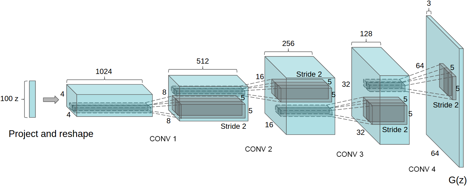
*Architecture of G using fractionally strided convolutions to progressively upscale the image.*


### Results
  * High quality images. Still with distortions and errors, but at first glance they look realistic.
  * Smooth interpolations between generated images are possible (by interpolating between the noise vectors and feeding these interpolations into G).
  * The features extracted by D seem to have some potential for unsupervised learning.
  * There seems to be some potential for vector arithmetics (using the initial noise vectors) similar to the vector arithmetics with wordvectors. E.g. to generate mean with sunglasses via `vector(men) + vector(sunglasses)`.


![Example images (bedrooms)](https://raw.githubusercontent.com/aleju/papers/master/neural-nets/images/Unsupervised_Representation_Learning_with_Deep_Convolutional_Generative_Adversarial_Networks__bedrooms.png?raw=true "Example images (bedrooms)")

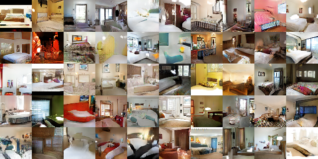*Generated images, bedrooms.*


![Example images (faces)](https://raw.githubusercontent.com/aleju/papers/master/neural-nets/images/Unsupervised_Representation_Learning_with_Deep_Convolutional_Generative_Adversarial_Networks__faces.png?raw=true "Example images (faces)")

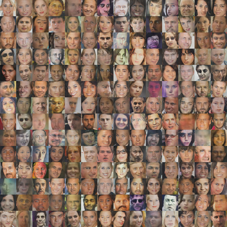*Generated images, faces.*



### Rough chapter-wise notes

* Introduction
  * For unsupervised learning, they propose to use to train a GAN and then reuse the weights of D.
  * GANs have traditionally been hard to train.

* Approach and model architecture
  * They use for D an convnet without linear layers, withput pooling layers (only strides), LeakyReLUs and Batch Normalization.
  * They use for G ReLUs (hidden layers) and Tanh (output).

* Details of adversarial training
  * They trained on LSUN, Imagenet-1k and a custom dataset of faces.
  * Minibatch size was 128.
  * LeakyReLU alpha 0.2.
  * They used Adam with a learning rate of 0.0002 and momentum of 0.5.
  * They note that a higher momentum lead to oscillations.

* LSUN
  * 3M images of bedrooms.
  * They use an autoencoder based technique to filter out 0.25M near duplicate images.

* Faces
  * They downloaded 3M images of 10k people.
  * They extracted 350k faces with OpenCV.

* Empirical validation of DCGANs capabilities
  * Classifying CIFAR-10 GANs as a feature extractor
    * They train a pair of G and D on Imagenet-1k.
    * D's top layer has `512*4*4` features.
    * They train an SVM on these features to classify the images of CIFAR-10.
    * They achieve a score of 82.8%, better than unsupervised K-Means based methods, but worse than Exemplar CNNs.
  * Classifying SVHN digits using GANs as a feature extractor
    * They reuse the same pipeline (D trained on CIFAR-10, SVM) for the StreetView House Numbers dataset.
    * They use 1000 SVHN images (with the features from D) to train the SVM.
    * They achieve 22.48% test error.

* Investigating and visualizing the internals of the networks
  * Walking in the latent space
    * The performs walks in the latent space (= interpolate between input noise vectors and generate several images for the interpolation).
    * They argue that this might be a good way to detect overfitting/memorizations as those might lead to very sudden (not smooth) transitions.
  * Visualizing the discriminator features
    * They use guided backpropagation to visualize what the feature maps in D have learned (i.e. to which images they react).
    * They can show that their LSUN-bedroom GAN seems to have learned in an unsupervised way what beds and windows look like.
  * Forgetting to draw certain objects
    * They manually annotated the locations of objects in some generated bedroom images.
    * Based on these annotations they estimated which feature maps were mostly responsible for generating the objects.
    * They deactivated these feature maps and regenerated the images.
    * That decreased the appearance of these objects. It's however not as easy as one feature map deactivation leading to one object disappearing. They deactivated quite a lot of feature maps (200) and they objects were often still quite visible or replaced by artefacts/errors.
  * Vector arithmetic on face samples
    * Wordvectors can be used to perform semantic arithmetic (e.g. `king - man + woman = queen`).
    * The unsupervised representations seem to be useable in a similar fashion.
    * E.g. they generated images via G. They then picked several images that showed men with glasses and averaged these image's noise vectors. They did with same with men without glasses and women without glasses. Then they performed on these vectors `men with glasses - mean without glasses + women without glasses` to get `woman with glasses