
|
Welcome to ShortScience.org! |


|
- ShortScience.org is a platform for post-publication discussion aiming to improve accessibility and reproducibility of research ideas.
- The website has 1584 public summaries, mostly in machine learning, written by the community and organized by paper, conference, and year.
- Reading summaries of papers is useful to obtain the perspective and insight of another reader, why they liked or disliked it, and their attempt to demystify complicated sections.
- Also, writing summaries is a good exercise to understand the content of a paper because you are forced to challenge your assumptions when explaining it.
- Finally, you can keep up to date with the flood of research by reading the latest summaries on our Twitter and Facebook pages.
Conditional Image Generation with PixelCNN Decoders
Aaron van den Oord and Nal Kalchbrenner and Oriol Vinyals and Lasse Espeholt and Alex Graves and Koray Kavukcuoglu
arXiv e-Print archive - 2016 via Local arXiv
Keywords: cs.CV, cs.LG
First published: 2016/06/16 (10 years ago)
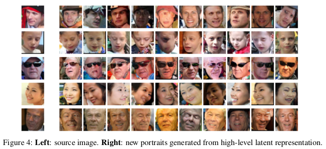
Abstract: This work explores conditional image generation with a new image density model based on the PixelCNN architecture. The model can be conditioned on any vector, including descriptive labels or tags, or latent embeddings created by other networks. When conditioned on class labels from the ImageNet database, the model is able to generate diverse, realistic scenes representing distinct animals, objects, landscapes and structures. When conditioned on an embedding produced by a convolutional network given a single image of an unseen face, it generates a variety of new portraits of the same person with different facial expressions, poses and lighting conditions. We also show that conditional PixelCNN can serve as a powerful decoder in an image autoencoder. Additionally, the gated convolutional layers in the proposed model improve the log-likelihood of PixelCNN to match the state-of-the-art performance of PixelRNN on ImageNet, with greatly reduced computational cost.
more
less
Aaron van den Oord and Nal Kalchbrenner and Oriol Vinyals and Lasse Espeholt and Alex Graves and Koray Kavukcuoglu
arXiv e-Print archive - 2016 via Local arXiv
Keywords: cs.CV, cs.LG
First published: 2016/06/16 (10 years ago)
Abstract: This work explores conditional image generation with a new image density model based on the PixelCNN architecture. The model can be conditioned on any vector, including descriptive labels or tags, or latent embeddings created by other networks. When conditioned on class labels from the ImageNet database, the model is able to generate diverse, realistic scenes representing distinct animals, objects, landscapes and structures. When conditioned on an embedding produced by a convolutional network given a single image of an unseen face, it generates a variety of new portraits of the same person with different facial expressions, poses and lighting conditions. We also show that conditional PixelCNN can serve as a powerful decoder in an image autoencoder. Additionally, the gated convolutional layers in the proposed model improve the log-likelihood of PixelCNN to match the state-of-the-art performance of PixelRNN on ImageNet, with greatly reduced computational cost.


[link]
* PixelRNN
* PixelRNNs generate new images pixel by pixel (and row by row) via LSTMs (or other RNNs).
* Each pixel is therefore conditioned on the previously generated pixels.
* Training of PixelRNNs is slow due to the RNN-architecture (hard to parallelize).
* Previously PixelCNNs have been suggested, which use masked convolutions during training (instead of RNNs), but their image quality was worse.
* They suggest changes to PixelCNNs that improve the quality of the generated images (while still keeping them faster than RNNs).
### How
* PixelRNNs split up the distribution `p(image)` into many conditional probabilities, one per pixel, each conditioned on all previous pixels: `p(image) = <product> p(pixel i | pixel 1, pixel 2, ..., pixel i-1)`.
* PixelCNNs implement that using convolutions, which are faster to train than RNNs.
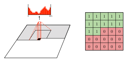
* These convolutions uses masked filters, i.e. the center weight and also all weights right and/or below the center pixel are `0` (because they are current/future values and we only want to condition on the past).
* In most generative models, several layers are stacked, ultimately ending in three float values per pixel (RGB images, one value for grayscale images). PixelRNNs (including this implementation) traditionally end in a softmax over 255 values per pixel and channel (so `3*255` per RGB pixel).
* The following image shows the application of such a convolution with the softmax output (left) and the mask for a filter (right):
* 
* Blind spot
* Using the mask on each convolutional filter effectively converts them into non-squared shapes (the green values in the image).
* Advantage: Using such non-squared convolutions prevents future values from leaking into present values.
* Disadvantage: Using such non-squared convolutions creates blind spots, i.e. for each pixel, some past values (diagonally top-right from it) cannot influence the value of that pixel.
* 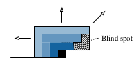
* They combine horizontal (1xN) and vertical (Nx1) convolutions to prevent that.
* Gated convolutions
* PixelRNNs via LSTMs so far created visually better images than PixelCNNs.
* They assume that one advantage of LSTMs is, that they (also) have multiplicative gates, while stacked convolutional layers only operate with summations.
* They alleviate that problem by adding gates to their convolutions:
* Equation: `output image = tanh(weights_1 * image) <element-wise product> sigmoid(weights_2 * image)`
* `*` is the convolutional operator.
* `tanh(weights_1 * image)` is a classical convolution with tanh activation function.
* `sigmoid(weights_2 * image)` are the gate values (0 = gate closed, 1 = gate open).
* `weights_1` and `weights_2` are learned.
* Conditional PixelCNNs
* When generating images, they do not only want to condition the previous values, but also on a laten vector `h` that describes the image to generate.
* The new image distribution becomes: `p(image) = <product> p(pixel i | pixel 1, pixel 2, ..., pixel i-1, h)`.
* To implement that, they simply modify the previously mentioned gated convolution, adding `h` to it:
* Equation: `output image = tanh(weights_1 * image + weights_2 . h) <element-wise product> sigmoid(weights_3 * image + weights_4 . h)`
* `.` denotes here the matrix-vector multiplication.
* PixelCNN Autoencoder
* The decoder in a standard autoencoder can be replaced by a PixelCNN, creating a PixelCNN-Autoencoder.
### Results
* They achieve similar NLL-results as PixelRNN on CIFAR-10 and ImageNet, while training about twice as fast.
* Here, "fast" means that they used 32 GPUs for 60 hours.
* Using Conditional PixelCNNs on ImageNet (i.e. adding class information to each convolution) did not improve the NLL-score, but it did improve the image quality.
* 
* They use a different neural network to create embeddings of human faces. Then they generate new faces based on these embeddings via PixelCNN.
* 
* Their PixelCNN-Autoencoder generates significantly sharper (i.e. less blurry) images than a "normal" autoencoder.
 |

InfoGAN: Interpretable Representation Learning by Information Maximizing Generative Adversarial Nets
Chen, Xi and Chen, Xi and Duan, Yan and Houthooft, Rein and Schulman, John and Sutskever, Ilya and Abbeel, Pieter
Neural Information Processing Systems Conference - 2016 via Local Bibsonomy
Keywords: dblp
Chen, Xi and Chen, Xi and Duan, Yan and Houthooft, Rein and Schulman, John and Sutskever, Ilya and Abbeel, Pieter
Neural Information Processing Systems Conference - 2016 via Local Bibsonomy
Keywords: dblp
|
[link]
* Usually GANs transform a noise vector `z` into images. `z` might be sampled from a normal or uniform distribution.
* The effect of this is, that the components in `z` are deeply entangled.
* Changing single components has hardly any influence on the generated images. One has to change multiple components to affect the image.
* The components end up not being interpretable. Ideally one would like to have meaningful components, e.g. for human faces one that controls the hair length and a categorical one that controls the eye color.
* They suggest a change to GANs based on Mutual Information, which leads to interpretable components.
* E.g. for MNIST a component that controls the stroke thickness and a categorical component that controls the digit identity (1, 2, 3, ...).
* These components are learned in a (mostly) unsupervised fashion.
### How
* The latent code `c`
* "Normal" GANs parameterize the generator as `G(z)`, i.e. G receives a noise vector and transforms it into an image.
* This is changed to `G(z, c)`, i.e. G now receives a noise vector `z` and a latent code `c` and transforms both into an image.
* `c` can contain multiple variables following different distributions, e.g. in MNIST a categorical variable for the digit identity and a gaussian one for the stroke thickness.
* Mutual Information
* If using a latent code via `G(z, c)`, nothing forces the generator to actually use `c`. It can easily ignore it and just deteriorate to `G(z)`.
* To prevent that, they force G to generate images `x` in a way that `c` must be recoverable. So, if you have an image `x` you must be able to reliable tell which latent code `c` it has, which means that G must use `c` in a meaningful way.
* This relationship can be expressed with mutual information, i.e. the mutual information between `x` and `c` must be high.
* The mutual information between two variables X and Y is defined as `I(X; Y) = entropy(X) - entropy(X|Y) = entropy(Y) - entropy(Y|X)`.
* If the mutual information between X and Y is high, then knowing Y helps you to decently predict the value of X (and the other way round).
* If the mutual information between X and Y is low, then knowing Y doesn't tell you much about the value of X (and the other way round).
* The new GAN loss becomes `old loss - lambda * I(G(z, c); c)`, i.e. the higher the mutual information, the lower the result of the loss function.
* Variational Mutual Information Maximization
* In order to minimize `I(G(z, c); c)`, one has to know the distribution `P(c|x)` (from image to latent code), which however is unknown.
* So instead they create `Q(c|x)`, which is an approximation of `P(c|x)`.
* `I(G(z, c); c)` is then computed using a lower bound maximization, similar to the one in variational autoencoders (called "Variational Information Maximization", hence the name "InfoGAN").
* Basic equation: `LowerBoundOfMutualInformation(G, Q) = E[log Q(c|x)] + H(c) <= I(G(z, c); c)`
* `c` is the latent code.
* `x` is the generated image.
* `H(c)` is the entropy of the latent codes (constant throughout the optimization).
* Optimization w.r.t. Q is done directly.
* Optimization w.r.t. G is done via the reparameterization trick.
* If `Q(c|x)` approximates `P(c|x)` *perfectly*, the lower bound becomes the mutual information ("the lower bound becomes tight").
* In practice, `Q(c|x)` is implemented as a neural network. Both Q and D have to process the generated images, which means that they can share many convolutional layers, significantly reducing the extra cost of training Q.
### Results
* MNIST
* They use for `c` one categorical variable (10 values) and two continuous ones (uniform between -1 and +1).
* InfoGAN learns to associate the categorical one with the digit identity and the continuous ones with rotation and width.
* Applying Q(c|x) to an image and then classifying only on the categorical variable (i.e. fully unsupervised) yields 95% accuracy.
* Sampling new images with exaggerated continuous variables in the range `[-2,+2]` yields sound images (i.e. the network generalizes well).
* 
* 3D face images
* InfoGAN learns to represent the faces via pose, elevation, lighting.
* They used five uniform variables for `c`. (So two of them apparently weren't associated with anything sensible? They are not mentioned.)
* 3D chair images
* InfoGAN learns to represent the chairs via identity (categorical) and rotation or width (apparently they did two experiments).
* They used one categorical variable (four values) and one continuous variable (uniform `[-1, +1]`).
* SVHN
* InfoGAN learns to represent lighting and to spot the center digit.
* They used four categorical variables (10 values each) and two continuous variables (uniform `[-1, +1]`). (Again, a few variables were apparently not associated with anything sensible?)
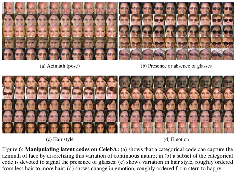
* CelebA
* InfoGAN learns to represent pose, presence of sunglasses (not perfectly), hair style and emotion (in the sense of "smiling or not smiling").
* They used 10 categorical variables (10 values each). (Again, a few variables were apparently not associated with anything sensible?)
* 
|
Improved Techniques for Training GANs
Salimans, Tim and Goodfellow, Ian J. and Zaremba, Wojciech and Cheung, Vicki and Radford, Alec and Chen, Xi
arXiv e-Print archive - 2016 via Local Bibsonomy
Keywords: dblp
Salimans, Tim and Goodfellow, Ian J. and Zaremba, Wojciech and Cheung, Vicki and Radford, Alec and Chen, Xi
arXiv e-Print archive - 2016 via Local Bibsonomy
Keywords: dblp
|
[link]
* They suggest some small changes to the GAN training scheme that lead to visually improved results.
* They suggest a new scoring method to compare the results of different GAN models with each other.
### How
* Feature Matching
* Usually G would be trained to mislead D as often as possible, i.e. to maximize D's output.
* Now they train G to minimize the feature distance between real and fake images. I.e. they do:
1. Pick a layer $l$ from D.
2. Forward real images through D and extract the features from layer $l$.
3. Forward fake images through D and extract the features from layer $l$.
4. Compute the squared euclidean distance between the layers and backpropagate.
* Minibatch discrimination
* They allow D to look at multiple images in the same minibatch.
* That is, they feed the features (of each image) extracted by an intermediate layer of D through a linear operation, resulting in a matrix per image.
* They then compute the L1-distances between these matrices.
* They then let D make its judgement (fake/real image) based on the features extracted from the image and these distances.
* They add this mechanism so that the diversity of images generated by G increases (which should also prevent collapses).
* Historical averaging
* They add a penalty term that punishes weights which are rather far away from their historical average values.
* I.e. the cost is `distance(current parameters, average of parameters over the last t batches)`.
* They argue that this can help the network to find equilibria that normal gradient descent would not find.
* One-sided label smoothing
* Usually one would use the labels 0 (image is fake) and 1 (image is real).
* Using smoother labels (0.1 and 0.9) seems to make networks more resistent to adversarial examples.
* So they smooth the labels of real images (apparently to 0.9?).
* Smoothing the labels of fake images would lead to (mathematical) problems in some cases, so they keep these at 0.
* Virtual Batch Normalization (VBN)
* Usually BN normalizes each example with respect to the other examples in the same batch.
* They instead normalize each example with respect to the examples in a reference batch, which was picked once at the start of the training.
* VBN is intended to reduce the dependence of each example on the other examples in the batch.
* VBN is computationally expensive, because it requires forwarding of two minibatches.
* They use VBN for their G.
* Inception Scoring
* They introduce a new scoring method for GAN results.
* Their method is based on feeding the generated images through another network, here they use Inception.
* For an image `x` and predicted classes `y` (softmax-output of Inception):
* They argue that they want `p(y|x)` to have low entropy, i.e. the model should be rather certain of seeing a class (or few classes) in the image.
* They argue that they want `p(y)` to have high entropy, i.e. the predicted classes (and therefore image contents) should have high diversity. (This seems like something that is quite a bit dependend on the used dataset?)
* They combine both measurements to the final score of `exp(KL(p(y|x) || p(y))) = exp( <sum over images> p(y|xi) * (log(p(y|xi)) - log(p(y))) )`.
* `p(y)` can be approximated as the mean of the softmax-outputs over many examples.
* Relevant python code that they use (where `part` seems to be of shape `(batch size, number of classes)`, i.e. the softmax outputs): `kl = part * (np.log(part) - np.log(np.expand_dims(np.mean(part, 0), 0))); kl = np.mean(np.sum(kl, 1)); scores.append(np.exp(kl));`
* They average this score over 50,000 generated images.
* Semi-supervised Learning
* For a dataset with K classes they extend D by K outputs (leading to K+1 outputs total).
* They then optimize two loss functions jointly:
* Unsupervised loss: The classic GAN loss, i.e. D has to predict the fake/real output correctly. (The other outputs seem to not influence this loss.)
* Supervised loss: D must correctly predict the image's class label, if it happens to be a real image and if it was annotated with a class.
* They note that training G with feature matching produces the best results for semi-supervised classification.
* They note that training G with minibatch discrimination produces significantly worse results for semi-supervised classification. (But visually the samples look better.)
* They note that using semi-supervised learning overall results in higher image quality than not using it. They speculate that this has to do with the class labels containing information about image statistics that are important to humans.
### Results
* MNIST
* They use weight normalization and white noise in D.
* Samples of high visual quality when using minibatch discrimination with semi-supervised learning.
* Very good results in semi-supervised learning when using feature matching.
* Using feature matching decreases visual quality of generated images, but improves results of semi-supervised learning.
* CIFAR-10
* D: 9-layer CNN with dropout, weight normalization.
* G: 4-layer CNN with batch normalization (so no VBN?).
* Visually very good generated samples when using minibatch discrimination with semi-supervised learning. (Probably new record quality.)
* Note: No comparison with nearest neighbours from the dataset.
* When using feature matching the results are visually not as good.
* Again, very good results in semi-supervised learning when using feature matching.
* SVHN
* Same setup as in CIFAR-10 and similar results.
* ImageNet
* They tried to generate 128x128 images and compared to DCGAN.
* They improved from "total garbage" to "garbage" (they now hit some textures, but structure is still wildly off).
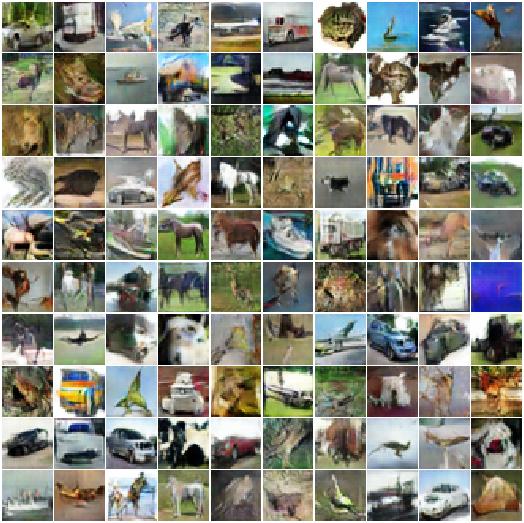
*Generated CIFAR-10-like images (with minibatch discrimination and semi-supervised learning).*
|
Synthesizing the preferred inputs for neurons in neural networks via deep generator networks
Nguyen, Anh and Dosovitskiy, Alexey and Yosinski, Jason and Brox, Thomas and Clune, Jeff
Neural Information Processing Systems Conference - 2016 via Local Bibsonomy
Keywords: dblp
Nguyen, Anh and Dosovitskiy, Alexey and Yosinski, Jason and Brox, Thomas and Clune, Jeff
Neural Information Processing Systems Conference - 2016 via Local Bibsonomy
Keywords: dblp
|
[link]
* They suggest a new method to generate images which maximize the activation of a specific neuron in a (trained) target network (abbreviated with "**DNN**").
* E.g. if your DNN contains a neuron that is active whenever there is a car in an image, the method should generate images containing cars.
* Such methods can be used to investigate what exactly a network has learned.
* There are plenty of methods like this one. They usually differ from each other by using different *natural image priors*.
* A natural image prior is a restriction on the generated images.
* Such a prior pushes the generated images towards realistic looking ones.
* Without such a prior it is easy to generate images that lead to high activations of specific neurons, but don't look realistic at all (e.g. they might look psychodelic or like white noise).
* That's because the space of possible images is extremely high-dimensional and can therefore hardly be covered reliably by a single network. Note also that training datasets usually only show a very limited subset of all possible images.
* Their work introduces a new natural image prior.
### How
* Usually, if one wants to generate images that lead to high activations, the basic/naive method is to:
1. Start with a noise image,
2. Feed that image through DNN,
3. Compute an error that is high if the activation of the specified neuron is low (analogous for high activation),
4. Backpropagate the error through DNN,
5. Change the noise image according to the gradient,
6. Repeat.
* So, the noise image is basically treated like weights in the network.
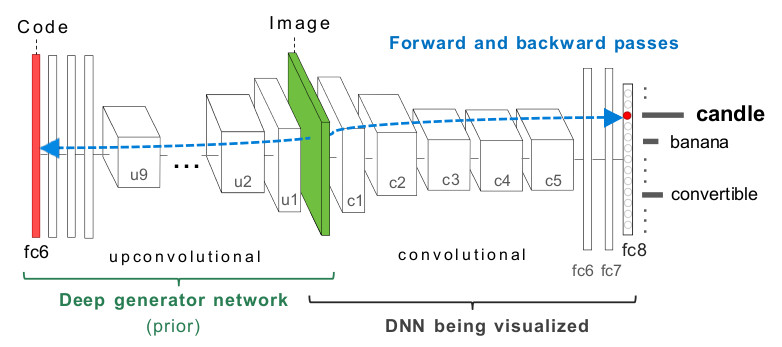
* Their alternative method is based on a Generator network **G**.
* That G is trained according to the method described in [Generating Images with Perceptual Similarity Metrics based on Deep Networks].
* Very rough outline of that method:
* First, a pretrained network **E** is given (they picked CaffeNet, which is a variation of AlexNet).
* G then has to learn to inverse E, i.e. G receives per image the features extracted by a specific layer in E (e.g. the last fully connected layer before the output) and has to generate (recreate) the image from these features.
* Their modified steps are:
1. *(New step)* Start with a noise vector,
2. *(New step)* Feed that vector through G resulting in an image,
3. *(Same)* Feed that image through DNN,
4. *(Same)* Compute an error that is low if the activation of the specified neuron is high (analogous for low activations),
5. *(Same)* Backpropagate the error through DNN,
6. *(Modified)* Change the noise *vector* according to the gradient,
7. *(Same)* Repeat.
* Visualization of their architecture:
* 
* Additionally they do:
* Apply an L2 norm to the noise vector, which adds pressure to each component to take low values. They say that this improved the results.
* Clip each component of the noise vector to a range `[0, a]`, which improved the results significantly.
* The range starts at `0`, because the network (E) inverted by their Generator (G) is based on ReLUs.
* `a` is derived from test images fed through E and set to 3 standard diviations of the mean activation of that component (recall that the "noise" vector mirrors a specific layer in E).
* They argue that this clipping is similar to a prior on the noise vector components. That prior reflects likely values of the layer in E that is used for the noise vector.
### Results
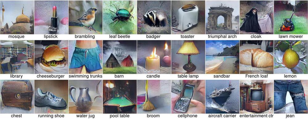
* Examples of generated images:
* 
* Early vs. late layers
* For G they have to pick a specific layer from E that G has to invert. They found that using "later" layers (e.g. the fully connected layers at the end) produced images with more reasonable overall structure than using "early" layers (e.g. first convolutional layers). Early layers led to repeating structures.
* Datasets and architectures
* Both G and DNN have to be trained on datasets.
* They found that these networks can actually be trained on different datasets, the results will still look good.
* However, they found that the architectures of DNN and E should be similar to create the best looking images (though this might also be down to depth of the tested networks).
* Verification that the prior can generate any image
* They tested whether the generated images really show what the DNN-neurons prefer and not what the Generator/prior prefers.
* To do that, they retrained DNNs on images that were both directly from the dataset as well as images that were somehow modified.
* Those modifications were:
* Treated RGB images as if they were BGR (creating images with weird colors).
* Copy-pasted areas in the images around (creating mosaics).
* Blurred the images (with gaussian blur).
* The DNNs were then trained to classify the "normal" images into 1000 classes and the modified images into 1000 other classes (2000 total).
* So at the end there were (in the same DNN) neurons reacting strongly to specific classes of unmodified images and other neurons that reacted strongly to specific classes of modified images.
* When generating images to maximize activations of specific neurons, the Generator was able to create both modified and unmodified images. Though it seemed to have some trouble with blurring.
* That shows that the generated images probably indeed show what the DNN has learned and not just what G has learned.
* Uncanonical images
* The method can sometimes generate uncanonical images (e.g. instead of a full dog just blobs of texture).
* They found that this seems to be mostly the case when the dataset images have uncanonical pose, i.e. are very diverse/multi-modal.
|
FractalNet: Ultra-Deep Neural Networks without Residuals
Larsson, Gustav and Maire, Michael and Shakhnarovich, Gregory
arXiv e-Print archive - 2016 via Local Bibsonomy
Keywords: dblp
Larsson, Gustav and Maire, Michael and Shakhnarovich, Gregory
arXiv e-Print archive - 2016 via Local Bibsonomy
Keywords: dblp
|
[link]
* They describe an architecture for deep CNNs that contains short and long paths. (Short = few convolutions between input and output, long = many convolutions between input and output)
* They achieve comparable accuracy to residual networks, without using residuals.
### How
* Basic principle:
* They start with two branches. The left branch contains one convolutional layer, the right branch contains a subnetwork.
* That subnetwork again contains a left branch (one convolutional layer) and a right branch (a subnetwork).
* This creates a recursion.
* At the last step of the recursion they simply insert two convolutional layers as the subnetwork.
* Each pair of branches (left and right) is merged using a pair-wise mean. (Result: One of the branches can be skipped or removed and the result after the merge will still be sound.)
* Their recursive expansion rule (left) and architecture (middle and right) visualized:

* Blocks:
* Each of the recursively generated networks is one block.
* They chain five blocks in total to create the network that they use for their experiments.
* After each block they add a max pooling layer.
* Their first block uses 64 filters per convolutional layer, the second one 128, followed by 256, 512 and again 512.
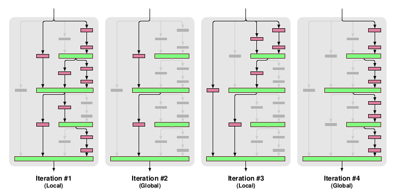
* Drop-path:
* They randomly dropout whole convolutional layers between merge-layers.
* They define two methods for that:
* Local drop-path: Drops each input to each merge layer with a fixed probability, but at least one always survives. (See image, first three examples.)
* Global drop-path: Drops convolutional layers so that only a single columns (and thereby path) in the whole network survives. (See image, right.)
* Visualization:
### Results
* They test on CIFAR-10, CIFAR-100 and SVHN with no or mild (crops, flips) augmentation.
* They add dropout at the start of each block (probabilities: 0%, 10%, 20%, 30%, 40%).
* They use for 50% of the batches local drop-path at 15% and for the other 50% global drop-path.
* They achieve comparable accuracy to ResNets (a bit behind them actually).
* Note: The best ResNet that they compare to is "ResNet with Identity Mappings". They don't compare to Wide ResNets, even though they perform best.
* If they use image augmentations, dropout and drop-path don't seem to provide much benefit (only small improvement).
* If they extract the deepest column and test on that one alone, they achieve nearly the same performance as with the whole network.
* They derive from that, that their fractal architecture is actually only really used to help that deepest column to learn anything. (Without shorter paths it would just learn nothing due to vanishing gradients.)
|