A finding first publicized by Geoff Hinton is the fact that, when you train a simple, lower capacity module on the probability outputs of another model, you can often get a model that has comparable performance, despite that lowered capacity. Another, even more interesting finding is that, if you take a trained model, and train a model with identical structure on its probability outputs, you can often get a model with better performance than the original teacher, with quicker convergence.

This paper addresses, and tries to specifically test, a few theories about why this effect might be observed. One idea is that the "student" model can learn more quickly because getting to see the full probability distribution over a well-trained models outputs gives it a more valuable signal, specifically because the trained model is able to better rank the classes that aren't the true class. For example, if you're training on Imagenet, on an image of a huskies, you're only told "this is a husky (1), and not one of 100 other classes, which are all 0". Whereas a trained model might say "'this is most likely a husky, but the probability of wolf is way higher than that of teapot". This inherently gives you more useful signal to train on, because you’re given a full distribution of classes that an image is most like. This theory goes by the name of the “Dark Knowledge” theory (a truly delightful name), because it pulls all of this knowledge that is hidden in a 0/1 label into the light. An alternative explanation for the strong performance of distillation techniques is that the student model is just benefitting from the implicit importance weighting of having a stronger gradient on examples where the teacher model is more confident. You could think of this as leading the student towards examples that are the most clear or unambiguous examples of a class, rather than more fuzzy and uncertain ones.

Along with a few other tests (which I won’t address here, for sake of time and focus), the authors design a few experiments to test these possible mechanisms of action. The first test involved doing an explicit importance weighting of examples according to how confident the teacher model is, but including no information about the incorrect classes. The second was similar, but instead involved perturbing the probabilities of the classes that weren’t the max probability. In this situation, the student model gets some information in terms of the overall magnitudes of the not-max class, but can’t leverage it as usefully because it’s been randomized.

In both situations, they found that there still was some value - in other words, that the student outperformed the teacher - but it outperformed by less than the case where the teacher could see the full probability distribution. This supports the case that both the inclusion of probabilities for the less probable classes, as well as the “confidence weighting” effect of weighting the student to learn more from examples on which the “teacher” model was more confident.

This is a nice little empirical paper that does some investigation into which features get learned during the course of neural network training. To look at this, it uses a notion of "decodability", defined as the accuracy to which you can train a linear model to predict a given conceptual feature on top of the activations/learned features at a particular layer. This idea captures the amount of information about a conceptual feature that can be extracted from a given set of activations. 

They work with two synthetic datasets. 

1. Trifeature: Generated images with a color, shape, and texture, which can be engineered to be either entirely uncorrelated or correlated with each other to varying degrees. 
2. Navon: Generated images that are letters on the level of shape, and are also composed of letters on the level of texture 

The first thing the authors investigate is: to what extent are the different properties of these images decodable from their representations, and how does that change during training? In general, decodability is highest in lower layers, and lowest in higher layers, which makes sense from the perspective of the Information Processing Inequality, since all the information is present in the pixels, and can only be lost in the course of training, not gained. They find that decodability of color is high, even in the later layers untrained networks, and that the decodability of texture and shape, while much less high, is still above chance. When the network is trained to predict one of the three features attached to an image, you see the decodability of that feature go up (as expected), but you also see the decodability of the other features go down, suggesting that training doesn't just involve amplifying predictive features, but also suppressing unpredictive ones. This effect is strongest in the Trifeature case when training for shape or color; when training for texture, the dampening effect on color is strong, but on shape is less pronounced. 

https://i.imgur.com/o45KHOM.png

The authors also performed some experiments on cases where features are engineered to be correlated to various degrees, to see which of the predictive features the network will represent more strongly. In the case where two features are perfectly correlated (and thus both perfectly predict the label), the network will focus decoding power on whichever feature had highest decodability in the untrained network, and, interestingly, will reduce decodability of the other feature (not just have it be lower than the chosen feature, but decrease it in the course of training), even though it is equally as predictive. 
https://i.imgur.com/NFx0h8b.png

Similarly, the network will choose the "easy" feature (the one more easily decodable at the beginning of training) even if there's another feature that is slightly *more* predictive available. This seems quite consistent with the results of another recent paper, Shah et al, on the Pitfalls of Simplicity Bias in neural networks. The overall message of both of these experiments is that networks generally 'put all their eggs in one basket,' so to speak, rather than splitting representational power across multiple features. 

There were a few other experiments in the paper, and I'd recommend reading it in full - it's quite well written - but I think those convey most of the key insights for me.

In response to increasing calls for ways to explain and interpret the predictions of neural networks, one major genre of explanation has been the construction of salience maps for image-based tasks. These maps assign a relevance or saliency score to every pixel in the image, according to various criteria by which the value of a pixel can be said to have influenced the final prediction of the network. This paper is an interesting blend of ideas from the saliency mapping literature with ones from adversarial examples: it essentially shows that you can create adversarial examples whose goal isn't to change the output of a classifier, but instead to keep the output of the classifier fixed, but radically change the explanation (their term for the previously-described pixel saliency map that results from various explanation-finding methods) to resemble some desired target explanation. This is basically a targeted adversarial example, but targeting a different property of the network (the calculated explanation) while keeping an additional one fixed (keeping the output of the original network close to the original output, as well as keeping the input image itself in a norm ball around the original image. This is done in a pretty standard way: by just defining a loss function incentivizing closeness to the original output and also closeness of the explanation to the desired target, and performing gradient descent to modify pixels until this loss was low. 

https://i.imgur.com/N9uReoJ.png

The authors do a decent job of showing such targeted perturbations are possible: by my assessment of their results their strongest successes at inducing an actual targeted explanation are with Layerwise Relevance Propogation and Pattern Attribution (two of the 6 tested explanation methods). With the other methods, I definitely buy that they're able to induce an explanation that's very unlike the true/original explanation, but it's not as clear they can reach an arbitrary target. This is a bit of squinting, but it seems like they have more success in influencing propogation methods (where the effect size of the output is propogated backwards through the network, accounting for ReLus) than they do with gradient ones (where you're simply looking at the gradient of the output class w.r.t each pixel. 

In the theory section of the paper, the authors do a bit of differential geometry that I'll be up front and say I did not have the niche knowledge to follow, but which essentially argues that the manipulability of an explanation has to do with the curvature of the output manifold for a constant output. That is to say: how much can you induce a large change in the gradient of the output, while moving a small distance along the manifold of a constant output value. They then go on to argue that ReLU activations, because they are by definition discontinuous, induce sharp changes in gradient for points nearby one another, and this increase the ability for networks to be manipulated. They propose a softplus activation instead, where instead of a sharp discontinuity, the ReLU shape becomes more curved, and show relatively convincingly that at low values of Beta (more curved) you can mostly eliminate the ability of a perturbation to induce an adversarially targeted explanation. 

https://i.imgur.com/Fwu3PXi.png

For all that I didn't have a completely solid grasp of some of the theory sections here, I think this is a neat proof of concept paper in showing that neural networks can be small-perturbation fragile on a lot of different axes: we've known this for a while in the area of adversarial examples, but this is a neat generalization of that fact to a new area.

Transformers - powered by self-attention mechanisms - have been a paradigm shift in NLP, and are now the standard choice for training large language models. However, while transformers do have many benefits in terms of computational constraints - most saliently, that attention between tokens can be computed in parallel, rather than needing to be evaluated sequentially like in a RNN - a major downside is their memory (and, secondarily, computational) requirements. The baseline form of self-attention works by having every token attend to every other token, where "attend" here means that a query from each token A will take an inner product with each other token -A, and then be elementwise-multiplied with the values of every other token -A. This implies a O(N^2) memory and computation requirement, where N is your sequence length. 

So, the question this paper asks is: how do you get the benefits, or most of the benefits, of a full-attention network, while reducing the number of other tokens each token attends to. 

The authors' solution - Big Bird - has three components. First, they approach the problem of approximating the global graph as a graph theory problem, where each token attending to every other is "fully connected," and the goal is to try to sparsify the graph in a way that keeps shortest path between any two nodes low. They use the fact that in an Erdos-Renyi graph - where very edge is simply chosen to be on or off with some fixed probability - the shortest path is known to be logN. In the context of aggregating information about a sequence, a short path between nodes means that the number of iterations, or layers, that it will take for information about any given node A to be part of the "receptive field" (so to speak) of node B, will be correspondingly short. Based on this, they propose having the foundation of their sparsified attention mechanism be simply a random graph, where each node attends to each other with probability k/N, where k is a tunable hyperparameter representing how many nodes each other node attends to on average. 

To supplement, the authors further note that sequence tasks of interest - particularly language - are very local in their information structure, and, while it's important to understand the global context of the full sequence, tokens close to a given token are most likely to be useful in constructing a representation of it. Given this, they propose supplementing their random-graph attention with a block diagonal attention, where each token attends to w/2 tokens prior to and subsequent to itself. (Where, again, w is a tunable hyperparameter) 

However, the authors find that these components aren't enough, and so they add a final component: having some small set of tokens that attend to all tokens, and are attended to by all tokens. This allows them to theoretically prove that Big Bird can approximate full sequences, and is a universal Turing machine, both of which are true for full Transformers. I didn't follow the details of the proof, but, intuitively, my reading of this is that having a small number of these global tokens basically acts as a shortcut way for information to get between tokens in the sequence - if information is globally valuable, it can be "written" to one of these global aggregator nodes, and then all tokens will be able to "read" it from there. 



The authors do note that while their sparse model approximates the full transformer well in many settings, there are some problems - like needing to find the token in the sequence that a given token is farthest from in vector space - that a full attention mechanism could solve easily (since it directly calculates all pairwise comparisons) but that a sparse attention mechanism would require many layers to calculate. 


Empirically, Big Bird ETC (a version which adds on additional tokens for the global aggregators, rather than making existing tokens serve thhttps://i.imgur.com/ks86OgJ.pnge purpose) performs the best on a big language model training objective, has comparable performance to existing models on questionhttps://i.imgur.com/x0BdamC.png answering, and pretty dramatic performance improvements in document summarization. It makes sense for summarization to be a place where this model in particular shines, because it's explicitly designed to be able to integrate information from very large contexts (albeit in a randomly sampled way), where full-attention architectures must, for reasons of memory limitation, do some variant of a sliding window approach.

  * They describe a model for human pose estimation, i.e. one that finds the joints ("skeleton") of a person in an image.
  * They argue that part of their model resembles a Markov Random Field (but in reality its implemented as just one big neural network).

### How
  * They have two components in their network:
    * Part-Detector:
      * Finds candidate locations for human joints in an image.
      * Pretty standard ConvNet. A few convolutional layers with pooling and ReLUs.
      * They use two branches: A fine and a coarse one. Both branches have practically the same architecture (convolutions, pooling etc.). The coarse one however receives the image downscaled by a factor of 2 (half width/height) and upscales it by a factor of 2 at the end of the branch.
      * At the end they merge the results of both branches with more convolutions.
      * The output of this model are 4 heatmaps (one per joint? unclear), each having lower resolution than the original image.
    * Spatial-Model:
      * Takes the results of the part detector and tries to remove all detections that were false positives.
      * They derive their architecture from a fully connected Markov Random Field which would be solved with one step of belief propagation.
      * They use large convolutions (128x128) to resemble the "fully connected" part.
      * They initialize the weights of the convolutions with joint positions gathered from the training set.
      * The convolutions are followed by log(), element-wise additions and exp() to resemble an energy function.
      * The end result are the input heatmaps, but cleaned up.

### Results
  * Beats all previous models (with and without spatial model).
  * Accuracy seems to be around 90% (with enough (16px) tolerance in pixel distance from ground truth).
  * Adding the spatial model adds a few percentage points of accuracy.
  * Using two branches instead of one (in the part detector) adds a bit of accuracy. Adding a third branch adds a tiny bit more.

![Results](https://raw.githubusercontent.com/aleju/papers/master/neural-nets/images/Joint_Training_of_a_ConvNet_and_a_PGM_for_HPE__results.png?raw=true "Results")

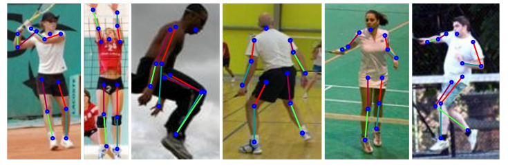
*Example results.*

![Part Detector](https://raw.githubusercontent.com/aleju/papers/master/neural-nets/images/Joint_Training_of_a_ConvNet_and_a_PGM_for_HPE__part_detector.png?raw=true "Part Detector")

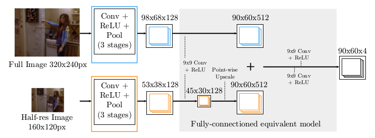
*Part Detector network.*

![Spatial Model](https://raw.githubusercontent.com/aleju/papers/master/neural-nets/images/Joint_Training_of_a_ConvNet_and_a_PGM_for_HPE__spatial_model.png?raw=true "Spatial Model")

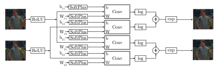
*Spatial Model (apparently only for two input heatmaps).*

-------------------------

# Rough chapter-wise notes

* (1) Introduction
  * Human Pose Estimation (HPE) from RGB images is difficult due to the high dimensionality of the input.
  * Approaches:
    * Deformable-part models: Traditionally based on hand-crafted features.
    * Deep-learning based disciminative models: Recently outperformed other models. However, it is hard to incorporate priors (e.g. possible joint- inter-connectivity) into the model.
  * They combine:
    * A part-detector (ConvNet, utilizes multi-resolution feature representation with overlapping receptive fields)
    * Part-based Spatial-Model (approximates loopy belief propagation)
  * They backpropagate through the spatial model and then the part-detector.

* (3) Model
  * (3.1) Convolutional Network Part-Detector
    * This model locates possible positions of human key joints in the image ("part detector").
    * Input: RGB image.
    * Output: 4 heatmaps, one per key joint (per pixel: likelihood).
    * They use a fully convolutional network.
    * They argue that applying convolutions to every pixel is similar to moving a sliding window over the image.
    * They use two receptive field sizes for their "sliding window": A large but coarse/blurry one, a small but fine one.
    * To implement that, they use two branches. Both branches are mostly identical (convolutions, poolings, ReLU). They simply feed a downscaled (half width/height) version of the input image into the coarser branch. At the end they upscale the coarser branch once and then merge both branches. 
    * After the merge they apply 9x9 convolutions and then 1x1 convolutions to get it down to 4xHxW (H=60, W=90 where expected input was H=320, W=240).
  * (3.2) Higher-level Spatial-Model
    * This model takes the detected joint positions (heatmaps) and tries to remove those that are probably false positives.
    * It is a ConvNet, which tries to emulate (1) a Markov Random Field and (2) solving that MRF approximately via one step of belief propagation.
    * The raw MRF formula would be something like `<likelihood of joint A per px> = normalize( <product over joint v from joints V> <probability of joint A per px given a> * <probability of joint v at px?> + someBiasTerm)`.
    * They treat the probabilities as energies and remove from the formula the partition function (`normalize`) for various reasons (e.g. because they are only interested in the maximum value anyways).
    * They use exp() in combination with log() to replace the product with a sum.
    * They apply SoftPlus and ReLU so that the energies are always positive (and therefore play well with log).
    * Apparently `<probability of joint v at px?>` are the input heatmaps of the part detector.
    * Apparently `<probability of joint A per px given a>` is implemented as the weights of a convolution.
    * Apparently `someBiasTerm` is implemented as the bias of a convolution.
    * The convolutions that they use are large (128x128) to emulate a fully connected graph.
    * They initialize the convolution weights based on histograms gathered from the dataset (empirical distribution of joint displacements).
  * (3.3) Unified Models
    * They combine the part-based model and the spatial model to a single one.
    * They first train only the part-based model, then only the spatial model, then both.

* (4) Results
  * Used datasets: FLIC (4k training images, 1k test, mostly front-facing and standing poses), FLIC-plus (17k, 1k ?), extended-LSP (10k, 1k).
  * FLIC contains images showing multiple persons with only one being annotated. So for FLIC they add a heatmap of the annotated body torso to the input (i.e. the part-detector does not have to search for the person any more).
  * The evaluation metric roughly measures, how often predicted joint positions are within a certain radius of the true joint positions.
  * Their model performs significantly better than competing models (on both FLIC and LSP).
  * Accuracy seems to be at around 80%-95% per joint (when choosing high enough evaluation tolerance, i.e. 10px+).
  * Adding the spatial model to the part detector increases the accuracy by around 10-15 percentage points.
  * Training the part detector and the spatial model jointly adds ~3 percentage points accuracy over training them separately.
  * Adding the second filter bank (coarser branch in the part detector) adds around 5 percentage points accuracy. Adding a third filter bank adds a tiny bit more accuracy.