The paper: "Deconstructing Lottery Tickets: Zeros, Signs, and the Supermask" by Zhou et al., 2019 found that by just learning binary masks one can find random subnetworks that do much better than chance on a task. This new paper builds on this method by proposing a strong algorithm than Zhou et al. for finding these high-performing subnetworks.https://i.imgur.com/vxDqCKP.png

The intuition follows: "If a neural network with random weights (center) is sufficiently overparameterized, it will contain a subnetwork (right) that performs as well as a trained neural network (left) with the same number of parameters."

While Zhou et al. learned a probability for each weight this paper learns a score for each weight and takes the top k percent at evaluation. The scores are learned through their primary contribution that they call the edge-popup algorithm: 

https://i.imgur.com/9KcIbxd.png

"In the edge-popup Algorithm, we associate a score with each edge. On the forward pass we choose the top edges by score. On the backward pass we update the scores of all the edges with the straight-through estimator, allowing helpful edges that are “dead” to re-enter the subnetwork. *We never update the value of any weight in the network, only the score associated with each weight.*"

They're able to find higher-performing random subnetworks than Zhou et al.

https://i.imgur.com/T3D7OsZ.png

This paper proposes a 3D human pose estimation in video method based on the dilated temporal convolutions applied on 2D keypoints (input to the network). 2D keypoints can be obtained using any person keypoint detector, but Mask R-CNN with ResNet-101 backbone, pre-trained on COCO and fine-tuned on 2D projections from Human3.6M, is used in the paper.
https://i.imgur.com/CdQONiN.png

The poses are presented as 2D keypoint coordinates in contrast to using heatmaps (i.e. Gaussian operation applied at the keypoint 2D location). Thus, 1D convolutions over the time series are applied, instead of 2D convolutions over heatmaps. The model is a fully convolutional architecture with residual connections that takes a sequence of 2D poses ( concatenated $(x,y)$ coordinates of the joints in each frame) as input and transforms them through temporal convolutions.
https://i.imgur.com/tCZvt6M.png
The `Slice` layer in the residual connection performs padding (or slicing) the sequence with replicas of boundary frames (to both left and right) to match the dimensions with the main block as zero-padding is not used in the convolution operations.

3D pose estimation is a difficult task particularly due to the limited data available online. Therefore, the authors propose semi-supervised approach of training the 2D->3D pose estimation by exploiting unlabeled video. Specifically, 2D keypoints are detected in the unlabeled video with any keypoint detector, then 3D keypoints are predicted from them and these 3D points are reprojected back to 2D (camera intrinsic parameters are required). This is idea similar to cycle consistency in the [CycleGAN](https://junyanz.github.io/CycleGAN/), for instance.
https://i.imgur.com/CBHxFOd.png
In the semi-supervised part (bottom part of the image above) training penalizes when the reprojected 2D keypoints are far from the original input. Weighted mean per-joint position error (WMPJPE) loss, weighted by the inverse of the depth to the object (since far objects should contribute less to the training than close ones) is used as the optimization goal.

The two networks (`supervised` above, `semi-supervised` below) have the same architecture but do not share any weights. They are jointly optimized where `semi-supervised` part serves as a regularizer. They communicate through the path aiming to make sure that the mean bone length of the above and below branches match.

The interesting tendency is observed from the MPJPE analysis with different amounts of supervised and unsupervised data available. Basically, the `semi-supervised` approach becomes more effective when less labeled data is available.
https://i.imgur.com/bHpVcSi.png

Additionally, the error is reduced when the ground truth keypoints are used. This means that a robust and accurate 2D keypoint detector is essential for the accurate 3D pose estimation in this setting.
https://i.imgur.com/rhhTDfo.png

This paper is a top-down (i.e. requires person detection separately) pose estimation method with a focus on improving high-resolution representations (features) to make keypoint detection easier. 

During the training stage, this method utilizes annotated bounding boxes of person class to extract ground truth images and keypoints. The data augmentations include random rotation, random scale, flipping, and [half body augmentations](http://presentations.cocodataset.org/ECCV18/COCO18-Keypoints-Megvii.pdf) (feeding upper or lower part of the body separately). Heatmap learning is performed in a typical for this task approach of applying L2 loss between predicted keypoint locations and ground truth locations (generated by applying 2D Gaussian with std = 1).

During the inference stage, pre-trained object detector is used to provide bounding boxes. The final heatmap is obtained by averaging heatmaps obtained from the original and flipped images. The pixel location of the keypoint is determined by $argmax$ heatmap value with a quarter offset in the direction to the second-highest heatmap value.

While the pipeline described in this paper is a common practice for pose estimation methods, this method can achieve better results by proposing a network design to extract better representations. This is done through having several parallel sub-networks of different resolutions (next one is half the size of the previous one) while repeatedly fusing branches between each other:
https://raw.githubusercontent.com/leoxiaobin/deep-high-resolution-net.pytorch/master/figures/hrnet.png

The fusion process varies depending on the scale of the sub-network and its location in relation to others:
https://i.imgur.com/mGDn7pT.png

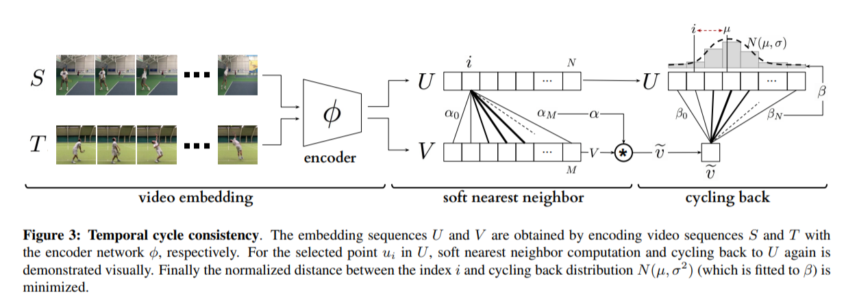
# Overview

This paper presents a novel way to align frames in videos of similar actions temporally in a self-supervised setting.  To do so, they leverage the concept of cycle-consistency. They introduce two formulations of cycle-consistency which are differentiable and solvable using standard gradient descent approaches. They name their method Temporal Cycle Consistency (TCC). They introduce a dataset that they use to evaluate their approach and show that their learned embeddings allow for few shot classification of actions from videos. 

Figure 1 shows the basic idea of what the paper aims to achieve. Given two video sequences, they wish to map the frames that are closest to each other in both sequences. The beauty here is that this "closeness" measure is defined by nearest neighbors in an embedding space, so the network has to figure out for itself what being close to another frame means. The cycle-consistency is what makes the network converge towards meaningful "closeness".

![image](https://user-images.githubusercontent.com/18450628/63888190-68b8a500-c9ac-11e9-9da7-925b72c731c3.png)

# Cycle Consistency

Intuitively, the concept of cycle-consistency can be thought of like this: suppose you have an application that allows you to take the photo of a user X and  increase their apparent age via some transformation F and decrease their age via some transformation G. The process is cycle-consistent if you can age your image, then using the aged image, "de-age" it and obtain something close to the original image you took; i.e. F(G(X))  ~= X.

In this paper, cycle-consistency is defined in the context of nearest-neighbors in the embedding space. Suppose you have two video sequences, U and V. Take a frame embedding from U, u_i, and find its nearest neighbor in V's embedding space, v_j. Now take the frame embedding v_j and find its closest frame embedding in U, u_k, using a nearest-neighbors approach. If k=i, the frames are cycle consistent. Otherwise, they are not. The authors seek to maximize cycle consistency across frames.
 
# Differentiable Cycle Consistency

The authors present two differentiable methods for cycle-consistency; cycle-back classification and cycle-back regression.

In order to make their cycle-consistency formulation differentiable, the authors use the concept of soft nearest neighbor:

![image](https://user-images.githubusercontent.com/18450628/63891061-5477a680-c9b2-11e9-9e4f-55e11d81787d.png)

## cycle-back classification

Once the soft nearest neighbor v~ is computed, the euclidean distance between v~ and all u_k  is computed for a total of N frames (assume N frames in U) in a logit vector x_k and softmaxed to a prediction ŷ = softmax(x): 

![image](https://user-images.githubusercontent.com/18450628/63891450-38c0d000-c9b3-11e9-89e9-d257be3fd175.png). 

![image](https://user-images.githubusercontent.com/18450628/63891746-e92ed400-c9b3-11e9-982c-078ebd1d747e.png)


Note the clever use of the negative, which will ensure the softmax selects for the highest distance. The ground truth label is a one-hot vector of size 1xN where position i is set to 1 and all others are set to 0. Cross-entropy is then used to compute the loss.

## cycle-back regression

The concept is very similar to cycle-back classification up to the soft nearest neighbor calculation. However the similarity metric of v~ back to u_k is not computed using euclidean distance but instead soft nearest neighbor again:

![image](https://user-images.githubusercontent.com/18450628/63893231-9bb46600-c9b7-11e9-9145-0c13e8ede5e6.png)

The idea is that they want to penalize the network less for "close enough" guesses. This is done by imposing a gaussian prior on beta centered around the actual closest neighbor i.

![image](https://user-images.githubusercontent.com/18450628/63893439-29905100-c9b8-11e9-81fe-fab238021c6d.png)

The following figure summarizes the pipeline:

![image](https://user-images.githubusercontent.com/18450628/63896278-9f4beb00-c9bf-11e9-8be1-5f1ad67199c7.png)

# Datasets

All training is done in a self-supervised fashion. To evaluate their methods, they annotate the Pouring dataset, which they introduce and the Penn Action dataset. To annotate the datasets, they limit labels to specific events and phases between phases 

![image](https://user-images.githubusercontent.com/18450628/63894846-affa6200-c9bb-11e9-8919-2f2cdf720a88.png)

# Model

The network consists of two parts: an encoder network and an embedder network.

## Encoder

They experiment with two encoders: 

* ResNet-50 pretrained on imagenet. They use conv_4 layer's output which is 14x14x1024 as the encoder scheme.

* A Vgg-like model from scratch whose encoder output is 14x14x512.

## Embedder

They then fuse the k following frame encodings along the time dimension, and feed it to an embedder network which uses 3D Convolutions and 3D pooling to reduce it to a 1x128 feature vector. They find that k=2 works pretty well.