[link]
Summary by Alexander Jung 7 years ago
* They compare the results of various models for pedestrian detection.
* The various models were developed over the course of ~10 years (2003-2014).
* They analyze which factors seemed to improve the results.
* They derive new models for pedestrian detection from that.
### Comparison: Datasets
* Available datasets
* INRIA: Small dataset. Diverse images.
* ETH: Video dataset. Stereo images.
* TUD-Brussels: Video dataset.
* Daimler: No color channel.
* Daimler stereo: Stereo images.
* Caltech-USA: Most often used. Large dataset.
* KITTI: Often used. Large dataset. Stereo images.
* All datasets except KITTI are part of the "unified evaluation toolbox" that allows authors to easily test on all of these datasets.
* The evaluation started initially with per-window (FPPW) and later changed to per-image (FPPI), because per-window skewed the results.
* Common evaluation metrics:
* MR: Log-average miss-rate (lower is better)
* AUC: Area under the precision-recall curve (higher is better)
### Comparison: Methods
* Families
* They identified three families of methods: Deformable Parts Models, Deep Neural Networks, Decision Forests.
* Decision Forests was the most popular family.
* No specific family seemed to perform better than other families.
* There was no evidence that non-linearity in kernels was needed (given sophisticated features).
* Additional data
* Adding (coarse) optical flow data to each image seemed to consistently improve results.
* There was some indication that adding stereo data to each image improves the results.
* Context
* For sliding window detectors, adding context from around the window seemed to improve the results.
* E.g. context can indicate whether there were detections next to the window as people tend to walk in groups.
* Deformable parts
* They saw no evidence that deformable part models outperformed other models.
* Multi-Scale models
* Training separate models for each sliding window scale seemed to improve results slightly.
* Deep architectures
* They saw no evidence that deep neural networks outperformed other models. (Note: Paper is from 2014, might have changed already?)
* Features
* Best performance was usually achieved with simple HOG+LUV features, i.e. by converting each window into:
* 6 channels of gradient orientations
* 1 channel of gradient magnitude
* 3 channels of LUV color space
* Some models use significantly more channels for gradient orientations, but there was no evidence that this was necessary to achieve good accuracy.
* However, using more different features (and more sophisticated ones) seemed to improve results.
### Their new model:
* They choose Decisions Forests as their model framework (2048 level-2 trees, i.e. 3 thresholds per tree).
* They use features from the [Integral Channels Features framework](http://pages.ucsd.edu/~ztu/publication/dollarBMVC09ChnFtrs_0.pdf). (Basically just a mixture of common/simple features per window.)
* They add optical flow as a feature.
* They add context around the window as a feature. (A second detector that detects windows containing two persons.)
* Their model significantly improves upon the state of the art (from 34 to 22% MR on Caltech dataset).
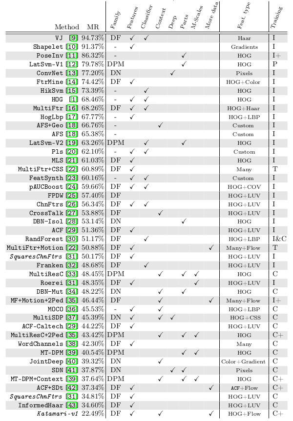
*Overview of models developed over the years, starting with Viola Jones (VJ) and ending with their suggested model (Katamari-v1). (DF = Decision Forest, DPM = Deformable Parts Model, DN = Deep Neural Network; I = Inria Dataset, C = Caltech Dataset)*


