If you’ve ever read a paper on Generative Adversarial Networks (from now on: GANs), you’ve almost certainly heard the author refer to the scourge upon the land of GANs that is mode collapse. When a generator succumbs to mode collapse, that means that, instead of modeling the full distribution, of input data, it will choose one region where there is a high density of data, and put all of its generated probability weight there. Then, on the next round, the discriminator pushes strongly away from that region (since it now is majority-occupied by fake data), and the generator finds a new mode. 

In the view of the authors of the Unrolled GANs paper,  one reason why this happens is that, in the typical GAN, at each round the generator implicitly assumes that it’s optimizing itself against the final and optimal discriminator. And, so, it makes its best move given that assumption, which is to put all its mass on a region the discriminator assigns high probability. Unfortunately for our short-sighted robot friend, this isn’t a one-round game, and this mass-concentrating strategy gives the discriminator a really good way to find fake data during the next round: just dramatically downweight how likely you think data is in the generator’s prior-round sweet spot, which it’s heavy concentration allows you to do without impacting your assessment of other data. Unrolled GANs operate on this key question: what if we could give the generator an ability to be less short-sighted, and make moves that aren’t just optimizing for the present, but are also defensive against the future, in ways that will hopefully tamp down on this running-around-in-circles dynamic illustrated above. If the generator was incentivized not only to make moves that fool the current discriminator, but also make moves that make the next-step discriminator less likely to tell it apart, the hope is that it will spread out its mass more, and be less likely to fall into the hole of a mode collapse. 

This intuition was realized in UnrolledGANs, through a mathematical approach that is admittedly a little complex for this discussion format. Essentially, in addition to the typical GAN loss (which is based on the current values of the generator and discriminator), this model also takes one “step forward” of the discriminator (calculates what the new parameters of the discriminator would be, if it took one update step), and backpropogates backward through that step. The loss under the next-step discriminator parameters is a function of both the current generator, and the next-step parameters, which come from the way the discriminator reacts to the current generator. When you take the gradient with respect to the generator of both of these things, you get something very like the ideal we described earlier: a generator that is trying to put its mass into areas the current discriminator sees as high-probability, but also change its parameters such that it gives the discriminator a less effective response strategy. 

https://i.imgur.com/0eEjm0g.png

Empirically: UnrolledGANs do a quite good job at their stated aim of reducing mode collapse, and the unrolled training procedure is now a common building-block technique used in other papers. 

_Objective:_ Fondamental analysis of random networks using mean-field theory. Introduces two scales controlling network behavior.

## Results:

Guide to choose hyper-parameters for random networks to be nearly critical (in between order and chaos). This in turn implies that information can propagate forward and backward and thus the network is trainable (not vanishing or exploding gradient).

Basically for any given number of layers and initialization covariances for weights and biases, tells you if the network will be trainable or not, kind of an architecture validation tool.

**To be noted:** any amount of dropout removes the critical point and therefore imply an upper bound on trainable network depth.

## Caveats:

*   Consider only bounded activation units: no relu, etc.
*   Applies directly only to fully connected feed-forward networks: no convnet, etc.

  * They describe an architecture for deep CNNs that contains short and long paths. (Short = few convolutions between input and output, long = many convolutions between input and output)
  * They achieve comparable accuracy to residual networks, without using residuals.

### How
  * Basic principle:
    * They start with two branches. The left branch contains one convolutional layer, the right branch contains a subnetwork.
    * That subnetwork again contains a left branch (one convolutional layer) and a right branch (a subnetwork).
    * This creates a recursion.
    * At the last step of the recursion they simply insert two convolutional layers as the subnetwork.
    * Each pair of branches (left and right) is merged using a pair-wise mean. (Result: One of the branches can be skipped or removed and the result after the merge will still be sound.)
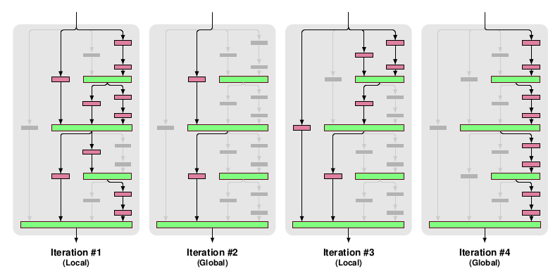
    * Their recursive expansion rule (left) and architecture (middle and right) visualized:
      ![Architecture](https://raw.githubusercontent.com/aleju/papers/master/neural-nets/images/FractalNet_Ultra-Deep_Networks_without_Residuals__architecture.png?raw=true "Architecture")
  * Blocks:
    * Each of the recursively generated networks is one block.
    * They chain five blocks in total to create the network that they use for their experiments.
    * After each block they add a max pooling layer.
    * Their first block uses 64 filters per convolutional layer, the second one 128, followed by 256, 512 and again 512.
  * Drop-path:
    * They randomly dropout whole convolutional layers between merge-layers.
    * They define two methods for that:
      * Local drop-path: Drops each input to each merge layer with a fixed probability, but at least one always survives. (See image, first three examples.)
      * Global drop-path: Drops convolutional layers so that only a single columns (and thereby path) in the whole network survives. (See image, right.)
    * Visualization:
      ![Drop-path](https://raw.githubusercontent.com/aleju/papers/master/neural-nets/images/FractalNet_Ultra-Deep_Networks_without_Residuals__drop_path.png?raw=true "Drop-path")

### Results
  * They test on CIFAR-10, CIFAR-100 and SVHN with no or mild (crops, flips) augmentation.
  * They add dropout at the start of each block (probabilities: 0%, 10%, 20%, 30%, 40%).
  * They use for 50% of the batches local drop-path at 15% and for the other 50% global drop-path.
  * They achieve comparable accuracy to ResNets (a bit behind them actually).
    * Note: The best ResNet that they compare to is "ResNet with Identity Mappings". They don't compare to Wide ResNets, even though they perform best.
  * If they use image augmentations, dropout and drop-path don't seem to provide much benefit (only small improvement).
  * If they extract the deepest column and test on that one alone, they achieve nearly the same performance as with the whole network.
    * They derive from that, that their fractal architecture is actually only really used to help that deepest column to learn anything. (Without shorter paths it would just learn nothing due to vanishing gradients.)

TLDR; The authors combine a standard LSTM softmax with [Pointer Networks](https://arxiv.org/abs/1506.03134) in a mixture model called Pointer-Sentinel LSTM (PS-LSTM). The pointer networks helps with rare words and long-term dependencies but is unable to refer to words that are not in the input. The oppoosite is the case for the standard softmax. By combining the two approaches we get the best of both worlds. The probability of an output words is defined as a mixture of the pointer and softmax model and the mixture coefficient is calculated as part of the pointer attention. The authors evaluate their architecture on the PTB Language Modeling dataset where they achieve state of the art. They also present a novel WikiText dataset that is larger and more realistic then PTB.


### Key Points:

- Standard RNNs with softmax struggle with rare and unseen words, even when adding attention.
- Use a window of the most recent`L` words to match against.
- Probability of output with gating: `p(y|x) = g * p_vocab(y|x) + (1 - g) * p_ptr(y|x)`.
- The gate `g` is calcualted as an extra element in the attention module. Probabilities for the pointer network are then normalized accordingly.
- Integrating the gating funciton computation into the pointer network is crucial: It needs to have access to the pointer network state, not just the RNN state (which can't hold long-term info)
- WikiText-2 dataset: 2M train tokens, 217k validation tokens, 245k test tokens. 33k vocab, 2.6% OOV. 2x larger than PTB.
- WikiText-1-3 dataset: 103M train tokens, 217k validation tokens, 245k test tokens. 267k vocab, 2.4% OOV. 100x larger than PTB.
- Pointer Sentiment Model leads to stronger improvements for rare words - that makes intuitive sense.

TLDR; The authors propose to use the Actor Critic framework from Reinforcement Learning for Sequence prediction. They train an actor (policy) network to generate a sequence together with a critic (value) network that estimates the q-value function. Crucially, the actor network does not see the ground-truth output, but the critic does. This is different from LL (log likelihood) where errors are likely to cascade. The authors evaluate their framework on an artificial spelling correction and a real-world German-English Machine Translation tasks, beating baselines and competing approaches in both cases.

#### Key Points

- In LL training, the model is conditioned on its own guesses during search, leading to error compounding.
- The critic is allowed to see the ground truth, but the actor isn't
- The reward is a task-specific score, e.g. BLEU
- Use bidirectional RNN for both actor and critic. Actor uses a soft attention mechanism.
- The reward is partially receives at each intermediate step, not just at the end
- Framework is analogous to TD-Learning in RL
- Trick: Use additional target network to compute q_t (see Deep-Q paper) for stability
- Trick: Use delayed actor (as in Deep Q paper) for stability
- Trick: Put constraint on critic to deal with large action spaces (is this analogous to advantage functions?)
- Pre-train actor and critic to encourage exploration of the right space
- Task 1: Correct corrupt character sequence. AC outperforms LL training. Longer sequences lead to stronger lift.
- Task 2: GER-ENG Machine Translation: Beats LL and Reinforce models
- Qualitatively, critic assigns high values to words that make sense
- BLUE scores during training are lower than those of LL model - Why? Strong regularization? Can't overfit the training data.

#### Notes

- Why does the sequence length for spelling prediction only go up to 30? This seems very short to me and something that an LSTM should be able to handle quite easily. Would've like to see much longer sequences.

TLDR; The authors augment the A3C (Asynchronous Actor Critic) algorithm with auxiliary tasks. These tasks share some of the network parameters but value functions for them are learned off-policy using n-step Q-Learning. The auxiliary tasks only used to learn a better representation and don't directly influence the main policy control. The technique, called UNREAL (Unsupervised Reinforcement and Auxiliary Learning), outperforms A3C on both the Atari and Labyrinth domains in terms of performance and training efficiency.


#### Key Points

- Environments contain a wide variety of possible training signals, not just cumulative reward
- Base A3C agent uses CNN + RNN
- Auxiliary Control and Prediction tasks share the convolutional and LSTM network for the "base agent". This forces the agent to balance improvement and base and aux. tasks.
- Auxiliary Tasks
  - Use off-policy RL algorithms (e.g. n-step Q-Learning) so that the same stream of experience from the base agent can be used for maximizing all tasks. Experience is sampled from a replay buffer.
  - Pixel Changes (Auxiliary Control): Learn a policy for maximally changing the pixels in a grid of cells overlaid over the images
  - Network Features (Auxiliary Control): Learn a policy for maximally activating units in a specific hidden layer
  - Reward Prediction (Auxiliary Reward): Predict the next reward given some historical context. Crucially, because rewards tend to be sparse, histories are sampled in a skewed manner from the replay buffer so that P(r!=0) = 0.5. Convolutional features are shared with the base agent.
  - Value Function Replay: Value function regression for the base agent with varying window for n-step returns.
- UNREAL
  - Base agent is optimized on-policy (A3C) and aux. tasks are optimized off-policy.
- Experiments
  - Agent is trained with 20-step returns and aux. tasks are performed every 20 steps.
  - Replay buffer stores the most recent 2k observations, actions and rewards
  - UNREAL tends to be more robust to hyperparameter settings than A3C
  - Labyrinth
    - 38% -> 83% human-normalized score. Each aux. tasks independently adds to the performance.
    - Significantly faster learning, 11x across all levels
    - Compared to input reconstruction technique: Input reconstruction hurts final performance b/c it puts too much focus on reconstructing relevant parts.
  - Atari
    - Not all experiments are completed yet, but UNREAL already surpasses state of the art agents and is more robust.

#### Thoughts

- I want an algorithm box please :)

This paper presents a way to differentiate through discrete random variables by replacing them with continuous random variables. Say you have a discrete [categorical variable][cat] and you're sampling it with the [Gumbel trick][gumbel] like this ($G_k$ is a Gumbel distributed variable and $\boldsymbol{\alpha}/\sum_k \alpha_k$ are our categorical probabilities):

$$
z = \text{one_hot} \left( \underset{k}{\text{arg max}} [ G_k + \log \alpha_k ] \right)
$$

This paper replaces the one hot and argmax with a softmax, and they add a $\lambda$ variable to control the "temperature". As $\lambda$ tends to zero it will equal the above equation.

$$
z = \text{softmax} \left( \frac{  G_k + \log \alpha_k }{\lambda} \right)
$$

I made [some notes][nb] on how this process works, if you'd like more intuition.

Comparison to [Gumbel-softmax][gs]
--------------------------------------------

These papers are proposed precisely the same distribution with notation changes ([noted there][gs]). Both papers also reference each other and the differences. Although, they mention differences in the variatonal objectives to the Gumbel-softmax. This paper also compares to [VIMCO][], which is probably a harder benchmark to compare against (multi-sample versus single sample).

The results in both papers compare to SOTA score function based estimators and both report high scoring results (often the best). There are some details about implementations to consider though, such as scheduling and exactly how to define the variational objective.

[cat]: https://en.wikipedia.org/wiki/Categorical_distribution
[gumbel]: https://hips.seas.harvard.edu/blog/2013/04/06/the-gumbel-max-trick-for-discrete-distributions/
[gs]: http://www.shortscience.org/paper?bibtexKey=journals/corr/JangGP16
[nb]: https://gist.github.com/gngdb/ef1999ce3a8e0c5cc2ed35f488e19748
[vimco]: https://arxiv.org/abs/1602.06725

This paper describes how to apply the idea of batch normalization (BN) successfully to recurrent neural networks, specifically to LSTM networks. The technique involves the 3 following ideas:

**1) Careful initialization of the BN scaling parameter.** While standard practice is to initialize it to 1 (to have unit variance), they show that this situation creates problems with the gradient flow through time, which vanishes quickly. A value around 0.1 (used in the experiments) preserves gradient flow much better.

**2) Separate BN for the "hiddens to hiddens pre-activation and for the "inputs to hiddens" pre-activation.** In other words, 2 separate BN operators are applied on each contributions to the pre-activation, before summing and passing through the tanh and sigmoid non-linearities.

**3) Use of largest time-step BN statistics for longer test-time sequences.** Indeed, one issue with applying BN to RNNs is that if the input sequences have varying length, and if one uses per-time-step mean/variance statistics in the BN transformation (which is the natural thing to do), it hasn't been clear how do deal with the last time steps of longer sequences seen at test time, for which BN has no statistics from the training set. The paper shows evidence that the pre-activation statistics tend to gradually converge to stationary values over time steps, which supports the idea of simply using the training set's last time step statistics.

Among these ideas, I believe the most impactful idea is 1). The papers mentions towards the end that improper initialization of the BN scaling parameter probably explains previous failed attempts to apply BN to recurrent networks.

Experiments on 4 datasets confirms the method's success.

**My two cents**

This is an excellent development for LSTMs. BN has had an important impact on our success in training deep neural networks, and this approach might very well have a similar impact on the success of LSTMs in practice.