# Summary

This paper presents state-of-the-art methods for both caption generation of images and visual question answering (VQA). The authors build on previous methods by adding what they call a "bottom-up" approach to previous "top-down" attention mechanisms. They show that using their approach they obtain SOTA on both Image captioning (MSCOCO) and the Visual Question and Answering (2017 VQA challenge). They propose a specific network configurations for each. Their biggest contribution is using Faster-R-CNN to retrieve the "important" parts of an image to focus on in both models.

## Top Down

Up until this paper, the traditional approach was to use a "top-down" approach, in which the last feature map layer of a CNN is used to obtain a latent representation of the given input image. These features, along with the context of the caption being generated, were used to generate attention weights that were used to predict the next sequence in the context of caption generation. The network would learn to focus its attention on regions of the feature map that matters most. This is the approach used in previous SOTA methods like [Show, Attend and Tell: Neural Image Caption Generation with Visual Attention](https://arxiv.org/abs/1502.03044).

## Bottom-up

The authors argue that the feature map of a CNN is too generic and can be thought of operating on a uniform, grid-like feature map. In other words, there is no particular reason to think that the feature map of generated by a CNN would give optimal regions to attend to. Also, carefully choosing the dimensions of the feature map can be very arbitrary.

In order to fix this, the authors propose combining object detection methods in a *bottom-up* approach. To do so, the authors propose using Faster-R-CNN to identify regions of interest in an image. Given an input image, Faster-R-CNN will identify bounding boxes of the image that likely correspond to objects of a given category and simultaneously compute a feature vector of that bounding box. Figure 1 shows the difference between the Bottom-up and Top-Down approach.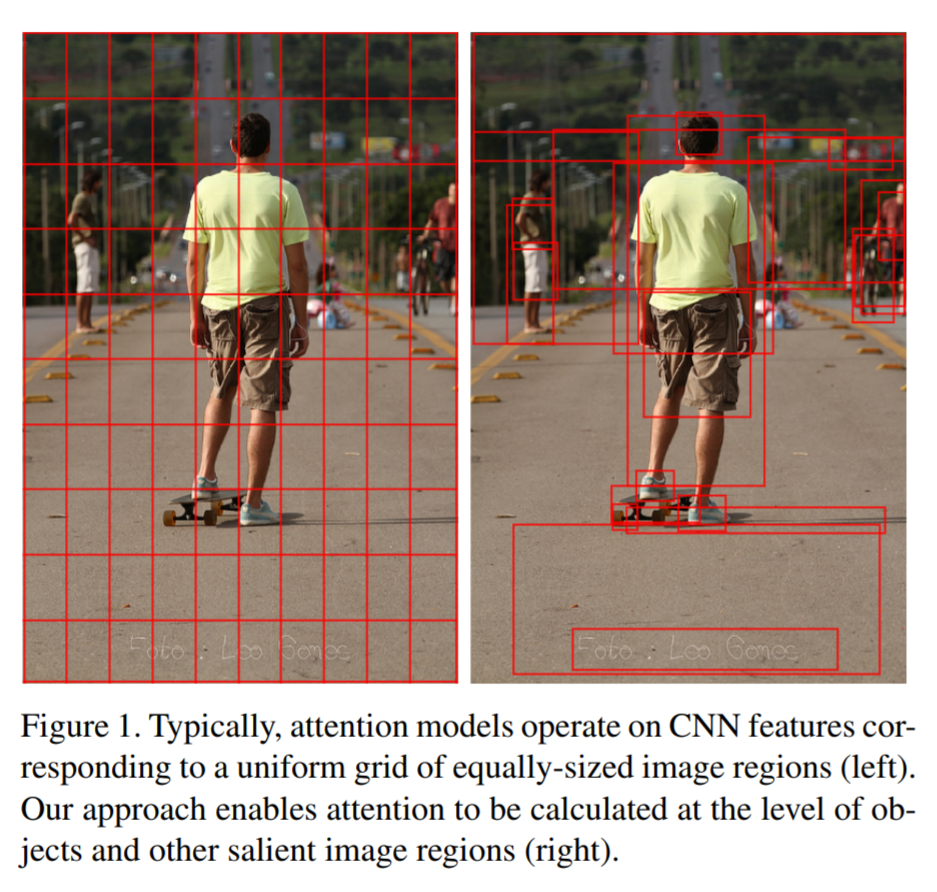

![image](https://user-images.githubusercontent.com/18450628/61817263-2683cd00-ae1c-11e9-971a-d3b531dbbd98.png)

## Combining the two

In this paper, the authors suggest using the bottom-up approach to compute the salient regions of the image the network should focus on using Faster-R-CNN. FRCNN is carefully pretrained on both imagenet and the Visual Genome dataset. It is then frozen and only used to generate bounding boxes of regions with high confidence of being of interest. The top-down approach is then used on the features obtained from the bottom-up approach. In order to "enhance" the FRCNN performance, they initialize their FRCNN with a ResNet-101 pre-trained on imagenet. They train their FRCNN on the Visual Genome dataset, adding attributes to the loss function that are available from the Visual Genome dataset, attributes such as color (black, white, gold etc.),  state (open, close, dark, bright, etc.). A sample of FRCNN outputs are shown in figure 2. It is important to stress that only the feature representations and not the actual outputs (i.e. not the labels) are used in their model.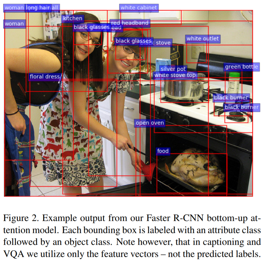

![image](https://user-images.githubusercontent.com/18450628/61817487-aca01380-ae1c-11e9-90fa-134033b95bb0.png)

## Caption Generation

Figure 3 provides a high-level overview of the model being used for caption generation for images. The image is first passed through FRCNN which produces a set of image features *V*. In their specific implementation, *V* consists of *k* vectors of size 1x2048. Their model consists of two LSTM blocks, one for attention and the other for language generation.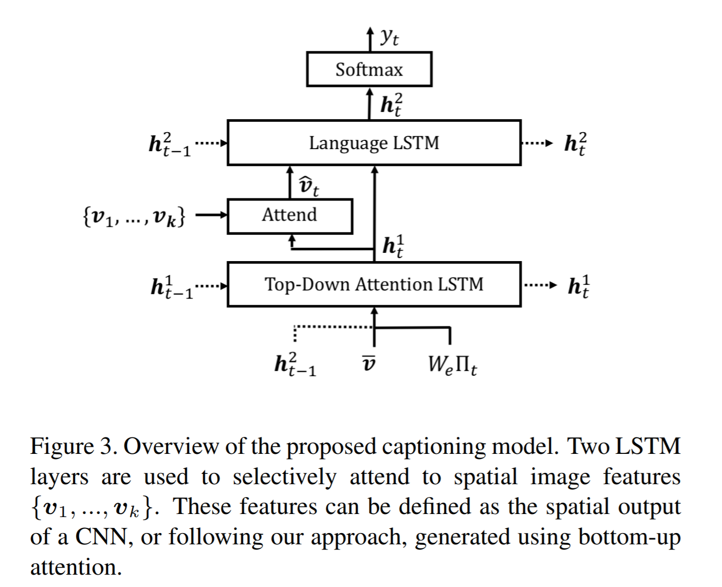

![image](https://user-images.githubusercontent.com/18450628/61818488-effb8180-ae1e-11e9-8ae4-14355115429a.png)

The first block of their model is a Top-Down Attention LSTM layer. It takes as input the mean-pooled features *V* , i.e. 1/k*sum(v_i), concatenated with the previous timestep's hidden representation of the language LSTM as well as the word embedding of the previously generated word. The word embedding is learned and not pretrained. 

The output of the first LSTM is used to compute the attention for each vector using an MLP and softmax: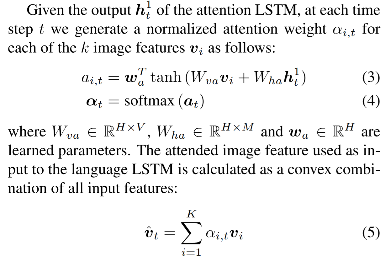

![image](https://user-images.githubusercontent.com/18450628/61819982-21298100-ae22-11e9-80a9-99640896413d.png)

The attention weighted image feature is then used as an input to the language LSTM model, concatenated with the output from the top-down Attention LSTM and a softmax is used to predict the next word in the sequence. The loss function seeks to minimize the cross-entropy of the generated sentence. 

## VQA Model

The VQA task differs to the image generation in that a text-based question accompanies an input image and the network must produce an answer. The VQA model proposed is different to that of the caption generation model previously described, however they both use the same bottom-up approach to generate the feature vectors of the image based on the FRCNN architecture. A high-level overview of the architecture for the VQA model is presented in Figure 4.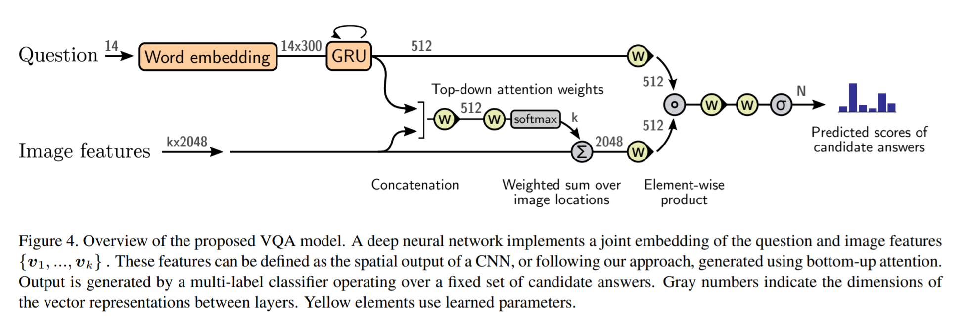

![image](https://user-images.githubusercontent.com/18450628/61821988-8da67f00-ae26-11e9-8456-3c9e5ec60787.png)

Each word from the question is converted to a learned word embedding which is used as input to a GRU. The number of words for each question is limited to 14 for computational efficiency. The output from the GRU is concatenated with each of the *k* image features, and attention weights are computed for each *k*th feature using an MLP and softmax, similar to what is done in the attention for caption generation. The weighted sum of the feature vectors is then passed through an linear layer such that its shape is compatible with the gru output, and the Hadamard product (element-wise product) is computed over the GRU output and attention-weighted image feature representation. Finally, a tanh non-linear activation is used. This results in a "gated tanh", which have been shown empirically to outperform both ReLU and tanh. Finally, a softmax probability distribution is generated at the output which selects a candidate answer among all possible candidate answers.

## Results and experiments

### Resnet Baseline

To demonstrate that their contribution of bottom-up mechanism actually improves on results, the authors use a ResNet trained on imagenet as a baseline for generating the image feature vectors (they resize the final CNN layers using bilinear interpolation when needed). They consistently obtain better results when using the bottom-up approach over the ResNet approach in both caption generation and VQA.

## MSCOCO

The authors demonstrate that they outperform all results on all metrics on the MSCOCO test server.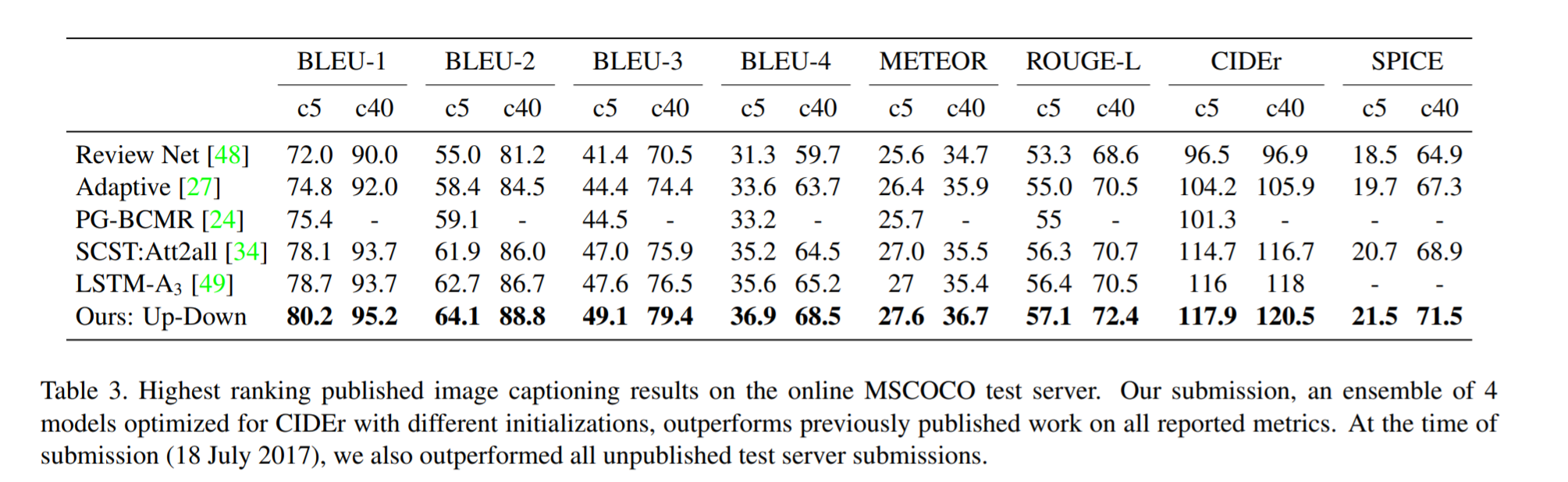

![image](https://user-images.githubusercontent.com/18450628/61824157-4f5f8e80-ae2b-11e9-8d90-657db453e26e.png)

They also show how using the bottom-up approach over ResNet consistently scores them higher on detecting instances of objects, attributes, relations, etc: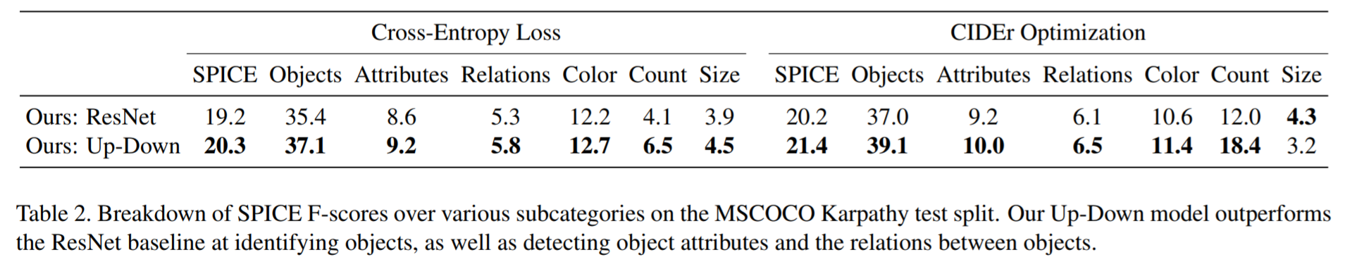

![image](https://user-images.githubusercontent.com/18450628/61824238-7fa72d00-ae2b-11e9-81b3-b5a7f80153f3.png)

The authors, like their predecessors, insist on demonstrating their network's frisbee ability: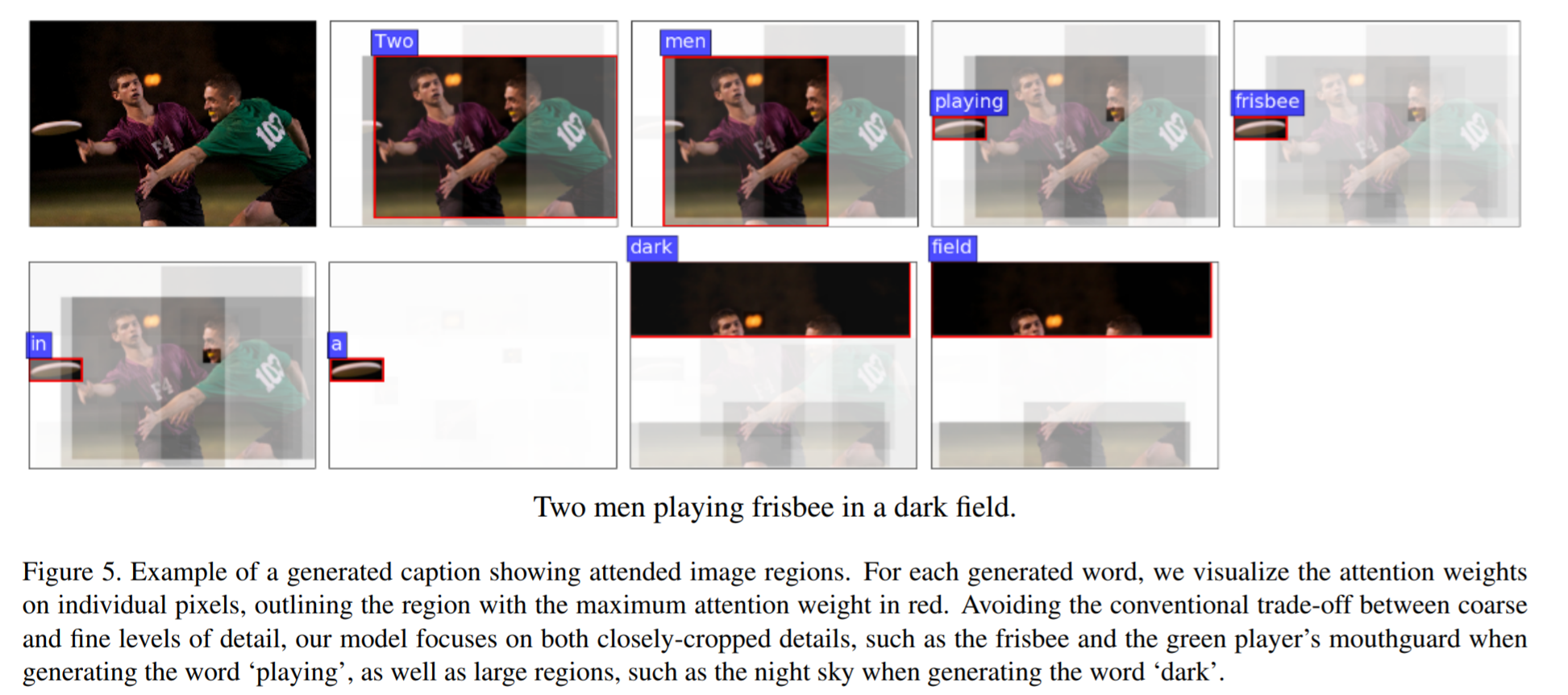

![image](https://user-images.githubusercontent.com/18450628/61824344-bed57e00-ae2b-11e9-87cd-597568587e1d.png)

## VQA Results

They also demonstrate that the addition of bottom-up attention improves results over a ResNet baseline.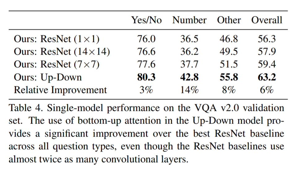 

![image](https://user-images.githubusercontent.com/18450628/61824500-28ee2300-ae2c-11e9-9016-2120a91917e4.png)

They also show that their model outperformed all other submissions on the VQA submission. They mention using an ensemble of 30 models for their submission.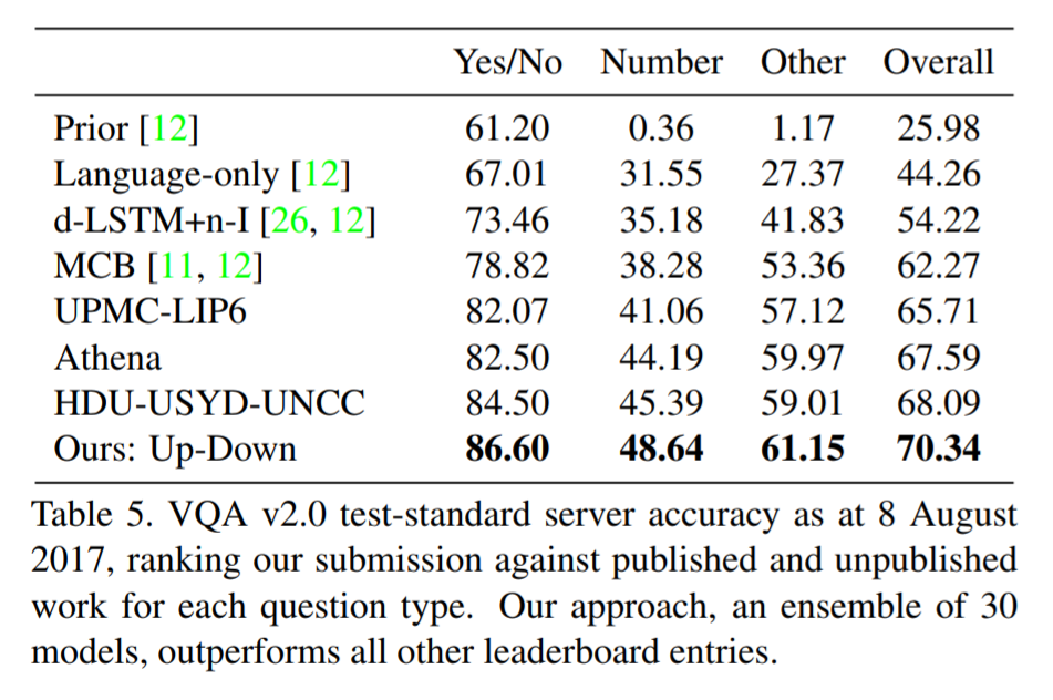 

![image](https://user-images.githubusercontent.com/18450628/61824634-83877f00-ae2c-11e9-8d84-9589e0ea2be2.png)


A sample image of what is attended in an image given a proper answer is shown in figure 6.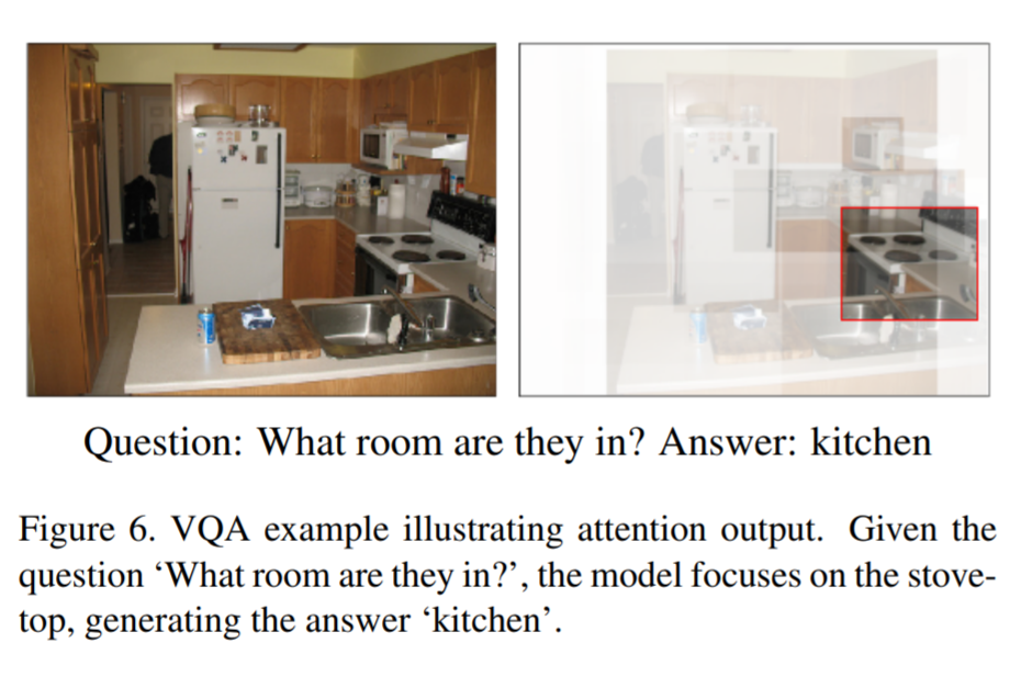

![image](https://user-images.githubusercontent.com/18450628/61824608-736f9f80-ae2c-11e9-9d4e-8cb6bd0a1a92.png)


# Comments

The authors introduce a new way to select portions of the image on which to focus attention. The idea is very original and came at a time when object detection was making significant progress (i.e. FRCNN).

A few comments:

* This method might not generalize well to other types of data. It requires pre-training on larger datasets (visual genome, imagenet, etc.) which consist of categories that overlap with both the MSCOCO and VQA datasets (i.e. cars, people, etc.). It would be interesting to see an end-to-end model that does not rely on pre-training on other similar datasets.

* No insight is given to the computational complexity nor to the inference time or training time. I imagine that FRCNN is resource intensive, and having to do a forward pass of FRCNN for every pass of the network must be a computational bottleneck. Not to mention that they ensembled 30 of them!

**TL;DR**: Rearranging the terms in Maximum Mean Discrepancy yields a much better loss function for the discriminator of Generative Adversarial Nets.

**Keywords**: Generative adversarial nets, Maximum Mean Discrepancy, spectral normalization, convolutional neural networks, Gaussian kernel, local stability.

**Summary**

Generative adversarial nets (GANs) are widely used to learn the data sampling process and are notoriously difficult to train. The training of GANs may be improved from three aspects: loss function, network architecture, and training process.

This study focuses on a loss function called the Maximum Mean Discrepancy (MMD), defined as:
$$
MMD^2(P_X,P_G)=\mathbb{E}_{P_X}k_{D}(x,x')+\mathbb{E}_{P_G}k_{D}(y,y')-2\mathbb{E}_{P_X,P_G}k_{D}(x,y)
$$
where $G,D$ are the generator and discriminator networks, $x,x'$ are real samples, $y,y'$ are generated samples, $k_D=k\circ D$ is a learned kernel that calculates the similariy between two samples. Overall, MMD calculates the distance between the real and the generated sample distributions. Thus, traditionally, the generator is trained to minimize $L_G=MMD^2(P_X,P_G)$, while the discriminator minimizes $L_D=-MMD^2(P_X,P_G)$.

This study makes three contributions:
-  It argues that $L_D$ encourages the discriminator to ignores the fine details in real data. By minimizing $L_D$, $D$ attempts to maximize $\mathbb{E}_{P_X}k_{D}(x,x')$, the similarity between real samples scores. Thus, $D$ has to focus on common features shared by real samples rather than fine details that separate them. This may slow down training. Instead, a repulsive loss is proposed, with no additional computational cost to MMD:
$$
L_D^{rep}=\mathbb{E}_{P_X}k_{D}(x,x')-\mathbb{E}_{P_G}k_{D}(y,y')
$$
- Inspired by the hinge loss, this study proposes a bounded Gaussian kernel for the discriminator to facilitate stable training of MMD-GAN.
- The spectral normalization method divides the weight matrix at each layer by its spectral norm to enforce that each layer is Lipschitz continuous. This study proposes a simple method to calculate the spectral norm of a convolutional kernel.

The results show the efficiency of proposed methods on CIFAR-10, STL-10, CelebA and LSUN-bedroom datasets. In Appendix, we prove that MMD-GAN training using gradient method is locally exponentially stable (a property that the Wasserstein loss does not have), and show that the repulsive loss works well with gradient penalty. 

The paper has been accepted at ICLR 2019 ([OpenReview link](https://openreview.net/forum?id=HygjqjR9Km)). The code is available at [GitHub link](https://github.com/richardwth/MMD-GAN). 

Lee et al. propose a regularizer to increase the size of linear regions of rectified deep networks around training and test points. Specifically, they assume piece-wise linear networks, in its most simplistic form consisting of linear layers (fully connected layers, convolutional layers) and ReLU activation functions. In these networks, linear regions are determined by activation patterns, i.e., a pattern indicating which neurons have value greater than zero. Then, the goal is to compute, and later to increase, the size $\epsilon$ such that the $L_p$-ball of radius $\epsilon$ around a sample $x$, denoted $B_{\epsilon,p}(x)$ is contained within one linear region (corresponding to one activation pattern). Formally, letting $S(x)$ denote the set of feasible inputs $x$ for a given activation pattern, the task is to determine

$\hat{\epsilon}_{x,p} = \max_{\epsilon \geq 0, B_{\epsilon,p}(x) \subset S(x)} \epsilon$.

For $p = 1, 2, \infty$, the authors show how $\hat{\epsilon}_{x,p}$ can be computed efficiently. For $p = 2$, for example, it results in

$\hat{\epsilon}_{x,p} = \min_{(i,j) \in I} \frac{|z_j^i|}{\|\nabla_x z_j^i\|_2}$.

Here, $z_j^i$ corresponds to the $j$th neuron in the $i$th layer of a multi-layer perceptron with ReLU activations; and $I$ contains all the indices of hidden neurons. This analytical form can then used to add a regularizer to encourage the network to learn larger linear regions:

$\min_\theta \sum_{(x,y) \in D} \left[\mathcal{L}(f_\theta(x), y) - \lambda \min_{(i,j) \in I} \frac{|z_j^i|}{\|\nabla_x z_j^i\|_2}\right]$

where $f_\theta$ is the neural network with paramters $\theta$. In the remainder of the paper, the authors propose a relaxed version of this training procedure that resembles a max-margin formulation and discuss efficient computation of the involved derivatives $\nabla_x z_j^i$ without too many additional forward/backward passes.

https://i.imgur.com/jSc9zbw.jpg
Figure 1: Visualization of locally linear regions for three different models on toy 2D data.

On toy data and datasets such as MNIST and CalTech-256, it is shown that the training procedure is effective in the sense that larger linear regions around training and test points are learned. For example, on a 2D toy dataset, Figure 1 visualizes the linear regions for the optimal regularizer as well as the proposed relaxed version.

Also find this summary at [davidstutz.de](https://davidstutz.de/category/reading/).

Offline reinforcement learning is potentially high-value thing for the machine learning community learn to do well, because there are many applications where it'd be useful to generate a learnt policy for responding to a dynamic environment, but where it'd be too unsafe or expensive to learn in an on-policy or online way, where we continually evaluate our actions in the environment to test their value. In such settings, we'd like to be able to take a batch of existing data - collected from a human demonstrator, or from some other algorithm - and be able to learn a policy from those pre-collected transitions, without being able to query the environment further by taking arbitrary actions. 

There are two broad strategies for learning a policy from precollected transitions. One is to simply learn to mimic the action policy used by the demonstrator, predicting the action the demonstrator would take in a given state, without making use of reward data at all. This is Behavioral Cloning, and has the advantage of being somewhat more conservative (in terms of not experimenting with possibly-unsafe-or-low-reward actions the demonstrator never took), but this is also a disadvantage, because it's not possible to get higher reward than the demonstrator themselves got if you're simply copying their behavior. Another approach is to learn a Q function - estimating the value of a given action in a given state - using the reward data from the precollected transitions. This can also have some downsides, mostly in the direction of overconfidence. Q value Temporal Difference learning works by using the current reward added to the max Q value over possible next actions as the target for the current-state Q estimate. This tends to lead to overestimates, because regression to the mean effects mean that the highest value Q estimates are disproportionately likely to be noisy (possibly because they correspond to an action with little data in the demonstrator dataset). In on-policy Q learning, this is less problematic, because the agent can take the action associated with their noisily inaccurate estimate, and as a result get more data for that action, and get an estimate that is less noisy in future. But when we're in a fully offline setting, all our learning is completed before we actually start taking actions with our policy, so taking high-uncertainty actions isn't a valuable source of new information, but just risky. 

The approach suggested by this DeepMind paper - Critic Regularized Regression, or CRR - is essentially a synthesis of these two possible approaches. The method learns a Q function as normal, using temporal difference methods. The distinction in this method comes from how to get a policy, given a learned Q function. Rather than simply taking the action your Q estimate says is highest-value at a particular point, CRR optimizes a policy according to the formula shown below. The f() function is a stand-in for various potential functions, all of which are monotonic with respect to the Q function, meaning they increase when the Q function does. 

https://i.imgur.com/jGmhYdd.png

This basically amounts to a form of a behavioral cloning loss (with the part that maximizes the probability under your policy of the actions sampled from the demonstrator dataset), but weighted or, as the paper terms it, filtered, by the learned Q function. The higher the estimated q value for a transition, the more weight is placed on that transition from the demo dataset having high probability under your policy. Rather than trying to mimic all of the actions of the demonstrator, the policy preferentially tries to mimic the demonstrator actions that it estimates were particularly high-quality. Different f() functions lead to different kinds of filtration. The `binary`version is an indicator function for the Advantage of an action (the Q value for that action at that state minus some reference value for the state, describing how much better the action is than other alternatives at that state) being greater than zero. Another, `exp`, uses exponential weightings which do a more "soft" upweighting or downweighting of transitions based on advantage, rather than the sharp binary of whether an actions advantage is above 1. 

The authors demonstrate that, on multiple environments from three different environment suites, CRR outperforms other off-policy baselines - either more pure behavioral cloning, or more pure RL - and in many cases does so quite dramatically. They find that the sharper binary weighting scheme does better on simpler tasks, since the trade-off of fewer but higher-quality samples to learn from works there. However, on more complex tasks, the policy benefits from the exp weighting, which still uses and learns from more samples (albeit at lower weights), which introduces some potential mimicking of lower-quality transitions, but at the trade of a larger effective dataset size to learn from.

Rakelly et al. propose a method to do off-policy meta reinforcement learning (rl). The method achieves a 20-100x improvement on sample efficiency compared to on-policy meta rl like MAML+TRPO. 

The key difficulty for offline meta rl arises from the meta-learning assumption, that meta-training and meta-test time match. However during test time the policy has to explore and sees as such on-policy data which is in contrast to the off-policy data that should be used at meta-training. The key contribution of PEARL is an algorithm that allows for online task inference in a latent variable at train and test time, which is used to train a Soft Actor Critic, a very sample efficient off-policy algorithm, with additional dependence of the latent variable.

The implementation of Rakelly et al. proposes to capture knowledge about the current task in a latent stochastic variable Z. A inference network $q_{\Phi}(z \vert c)$ is used to predict the posterior over latents given context c of the current task in from of transition tuples $(s,a,r,s')$ and trained with an information bottleneck. Note that the task inference is done on samples according to a sampling strategy sampling more recent transitions. The latent z is used as an additional input to policy $\pi(a \vert s, z)$ and Q-function $Q(a,s,z)$ of a soft actor critic algorithm which is trained with offline data of the full replay buffer. 

https://i.imgur.com/wzlmlxU.png 


So the challenge of differing conditions at test and train times is resolved by sampling the content for the latent context variable at train time only from very recent transitions (which is almost on-policy) and at test time by construction on-policy. Sampling $z \sim q(z \vert c)$ at test time allows for posterior sampling of the latent variable, yielding efficient exploration. 

The experiments are performed across 6 Mujoco tasks with ProMP, MAML+TRPO and $RL^2$ with PPO as baselines. They show:
- PEARL is 20-100x more sample-efficient 
- the posterior sampling of the latent context variable enables deep exploration that is crucial for sparse reward settings
- the inference network could be also a RNN, however it is crucial to train it with uncorrelated transitions instead of trajectories that have high correlated transitions
- using a deterministic latent variable, i.e. reducing $q_{\Phi}(z \vert c)$ to a  point estimate, leaves the algorithm unable to solve sparse reward navigation tasks which is attributed to the lack of temporally extended exploration. 

The paper introduces an algorithm that allows to combine meta learning with an off-policy algorithm that dramatically increases the sample-efficiency compared to on-policy meta learning approaches. This increases the chance of seeing meta rl in any sort of real world applications.