
|
Welcome to ShortScience.org! |


|
- ShortScience.org is a platform for post-publication discussion aiming to improve accessibility and reproducibility of research ideas.
- The website has 1584 public summaries, mostly in machine learning, written by the community and organized by paper, conference, and year.
- Reading summaries of papers is useful to obtain the perspective and insight of another reader, why they liked or disliked it, and their attempt to demystify complicated sections.
- Also, writing summaries is a good exercise to understand the content of a paper because you are forced to challenge your assumptions when explaining it.
- Finally, you can keep up to date with the flood of research by reading the latest summaries on our Twitter and Facebook pages.
Rich Feature Hierarchies for Accurate Object Detection and Semantic Segmentation
Girshick, Ross B. and Donahue, Jeff and Darrell, Trevor and Malik, Jitendra
Conference and Computer Vision and Pattern Recognition - 2014 via Local Bibsonomy
Keywords: dblp
Girshick, Ross B. and Donahue, Jeff and Darrell, Trevor and Malik, Jitendra
Conference and Computer Vision and Pattern Recognition - 2014 via Local Bibsonomy
Keywords: dblp


[link]
# Object detection system overview. https://i.imgur.com/vd2YUy3.png 1. takes an input image, 2. extracts around 2000 bottom-up region proposals, 3. computes features for each proposal using a large convolutional neural network (CNN), and then 4. classifies each region using class-specific linear SVMs. * R-CNN achieves a mean average precision (mAP) of 53.7% on PASCAL VOC 2010. * On the 200-class ILSVRC2013 detection dataset, R-CNN’s mAP is 31.4%, a large improvement over OverFeat , which had the previous best result at 24.3%. ## There is a 2 challenges faced in object detection 1. localization problem 2. labeling the data 1 localization problem : * One approach frames localization as a regression problem. they report a mAP of 30.5% on VOC 2007 compared to the 58.5% achieved by our method. * An alternative is to build a sliding-window detector. considered adopting a sliding-window approach increases the number of convolutional layers to 5, have very large receptive fields (195 x 195 pixels) and strides (32x32 pixels) in the input image, which makes precise localization within the sliding-window paradigm. 2 labeling the data: * The conventional solution to this problem is to use unsupervised pre-training, followed by supervise fine-tuning * supervised pre-training on a large auxiliary dataset (ILSVRC), followed by domain specific fine-tuning on a small dataset (PASCAL), * fine-tuning for detection improves mAP performance by 8 percentage points. * Stochastic gradient descent via back propagation was used to effective for training convolutional neural networks (CNNs) ## Object detection with R-CNN This system consists of three modules * The first generates category-independent region proposals. These proposals define the set of candidate detections available to our detector. * The second module is a large convolutional neural network that extracts a fixed-length feature vector from each region. * The third module is a set of class specific linear SVMs. Module design 1 Region proposals * which detect mitotic cells by applying a CNN to regularly-spaced square crops. * use selective search method in fast mode (Capture All Scales, Diversification, Fast to Compute). * the time spent computing region proposals and features (13s/image on a GPU or 53s/image on a CPU) 2 Feature extraction. * extract a 4096-dimensional feature vector from each region proposal using the Caffe implementation of the CNN * Features are computed by forward propagating a mean-subtracted 227x227 RGB image through five convolutional layers and two fully connected layers. * warp all pixels in a tight bounding box around it to the required size * The feature matrix is typically 2000x4096 3 Test time detection * At test time, run selective search on the test image to extract around 2000 region proposals (we use selective search’s “fast mode” in all experiments). * warp each proposal and forward propagate it through the CNN in order to compute features. Then, for each class, we score each extracted feature vector using the SVM trained for that class. * Given all scored regions in an image, we apply a greedy non-maximum suppression (for each class independently) that rejects a region if it has an intersection-over union (IoU) overlap with a higher scoring selected region larger than a learned threshold. ## Training 1 Supervised pre-training: * pre-trained the CNN on a large auxiliary dataset (ILSVRC2012 classification) using image-level annotations only (bounding box labels are not available for this data) 2 Domain-specific fine-tuning. * use the stochastic gradient descent (SGD) training of the CNN parameters using only warped region proposals with learning rate of 0.001. 3 Object category classifiers. * use intersection-over union (IoU) overlap threshold method to label a region with The overlap threshold of 0.3. * Once features are extracted and training labels are applied, we optimize one linear SVM per class. * adopt the standard hard negative mining method to fit large training data in memory. ### Results on PASCAL VOC 201012 1 VOC 2010 * compared against four strong baselines including SegDPM, DPM, UVA, Regionlets. * Achieve a large improvement in mAP, from 35.1% to 53.7% mAP, while also being much faster https://i.imgur.com/0dGX9b7.png 2 ILSVRC2013 detection. * ran R-CNN on the 200-class ILSVRC2013 detection dataset * R-CNN achieves a mAP of 31.4% https://i.imgur.com/GFbULx3.png #### Performance layer-by-layer, without fine-tuning 1 pool5 layer * which is the max pooled output of the network’s fifth and final convolutional layer. *The pool5 feature map is 6 x6 x 256 = 9216 dimensional * each pool5 unit has a receptive field of 195x195 pixels in the original 227x227 pixel input 2 Layer fc6 * fully connected to pool5 * it multiplies a 4096x9216 weight matrix by the pool5 feature map (reshaped as a 9216-dimensional vector) and then adds a vector of biases 3 Layer fc7 * It is implemented by multiplying the features computed by fc6 by a 4096 x 4096 weight matrix, and similarly adding a vector of biases and applying half-wave rectification #### Performance layer-by-layer, with fine-tuning * CNN’s parameters fine-tuned on PASCAL. * fine-tuning increases mAP by 8.0 % points to 54.2% ### Network architectures * 16-layer deep network, consisting of 13 layers of 3 _ 3 convolution kernels, with five max pooling layers interspersed, and topped with three fully-connected layers. We refer to this network as “O-Net” for OxfordNet and the baseline as “T-Net” for TorontoNet. * RCNN with O-Net substantially outperforms R-CNN with TNet, increasing mAP from 58.5% to 66.0% * drawback in terms of compute time, with in terms of compute time, with than T-Net. 1 The ILSVRC2013 detection dataset * dataset is split into three sets: train (395,918), val (20,121), and test (40,152) #### CNN features for segmentation. * full R-CNN: The first strategy (full) ignores the re region’s shape and computes CNN features directly on the warped window. Two regions might have very similar bounding boxes while having very little overlap. * fg R-CNN: the second strategy (fg) computes CNN features only on a region’s foreground mask. We replace the background with the mean input so that background regions are zero after mean subtraction. * full+fg R-CNN: The third strategy (full+fg) simply concatenates the full and fg features https://i.imgur.com/n1bhmKo.png 
1 Comments
 |

RandomOut: Using a convolutional gradient norm to win The Filter Lottery
Cohen, Joseph Paul and Lo, Henry Z. and Ding, Wei
arXiv e-Print archive - 2016 via Local Bibsonomy
Keywords: dblp
Cohen, Joseph Paul and Lo, Henry Z. and Ding, Wei
arXiv e-Print archive - 2016 via Local Bibsonomy
Keywords: dblp
|
[link]
Basically they observe a pattern they call The Filter Lottery (TFL) where the random seed causes a high variance in the training accuracy:

They use the convolutional gradient norm ($CGN$) \cite{conf/fgr/LoC015} to determine how much impact a filter has on the overall classification loss function by taking the derivative of the loss function with respect each weight in the filter.
$$CGN(k) = \sum_{i} \left|\frac{\partial L}{\partial w^k_i}\right|$$
They use the CGN to evaluate the impact of a filter on error, and re-initialize filters when the gradient norm of its weights falls below a specific threshold.
|

How Does Batch Normalization Help Optimization? (No, It Is Not About Internal Covariate Shift)
Shibani Santurkar and Dimitris Tsipras and Andrew Ilyas and Aleksander Madry
arXiv e-Print archive - 2018 via Local arXiv
Keywords: stat.ML, cs.LG, cs.NE
First published: 2018/05/29 (7 years ago)
Abstract: Batch Normalization (BatchNorm) is a widely adopted technique that enables faster and more stable training of deep neural networks (DNNs). Despite its pervasiveness, the exact reasons for BatchNorm's effectiveness are still poorly understood. The popular belief is that this effectiveness stems from controlling the change of the layers' input distributions during training to reduce the so-called "internal covariate shift". In this work, we demonstrate that such distributional stability of layer inputs has little to do with the success of BatchNorm. Instead, we uncover a more fundamental impact of BatchNorm on the training process: it makes the optimization landscape significantly smoother. This smoothness induces a more predictive and stable behavior of the gradients, allowing for faster training. These findings bring us closer to a true understanding of our DNN training toolkit.
more
less
Shibani Santurkar and Dimitris Tsipras and Andrew Ilyas and Aleksander Madry
arXiv e-Print archive - 2018 via Local arXiv
Keywords: stat.ML, cs.LG, cs.NE
First published: 2018/05/29 (7 years ago)
Abstract: Batch Normalization (BatchNorm) is a widely adopted technique that enables faster and more stable training of deep neural networks (DNNs). Despite its pervasiveness, the exact reasons for BatchNorm's effectiveness are still poorly understood. The popular belief is that this effectiveness stems from controlling the change of the layers' input distributions during training to reduce the so-called "internal covariate shift". In this work, we demonstrate that such distributional stability of layer inputs has little to do with the success of BatchNorm. Instead, we uncover a more fundamental impact of BatchNorm on the training process: it makes the optimization landscape significantly smoother. This smoothness induces a more predictive and stable behavior of the gradients, allowing for faster training. These findings bring us closer to a true understanding of our DNN training toolkit.
|
[link]
At NIPS 2017, Ali Rahimi was invited on stage to give a keynote after a paper he was on received the “Test of Time” award. While there, in front of several thousand researchers, he gave an impassioned argument for more rigor: more small problems to validate our assumptions, more visibility into why our optimization algorithms work the way they do. The now-famous catchphrase of the talk was “alchemy”; he argued that the machine learning community has been effective at finding things that work, but less effective at understanding why the techniques we use work. A central example he used in his talk is that of Batch Normalization: a now nearly-universal step in optimizing deep nets, but one where our accepted explanation of “reducing internal covariate shift” is less rigorous than one might hope.

With apologies for the long preamble, this is the context in which today’s paper is such a welcome push in the direction of what Rahimi was advocating for - small, focused experimentation that tries to build up knowledge from principles, and, specifically, asks the question: “Does Batch Norm really work via reducing covariate shift”.

To answer the question of whether internal covariate shift is a likely mechanism of the - empirically very solid - improved performance of Batch Norm, the authors do a few simple experience. First, and most straightforwardly, they train a basic convolutional net with and without BatchNorm, pick a layer, and visualize the activation distribution of that layer over time, both in the Batch Norm and non-Batch Norm case. While they saw the expected performance boost, the Batch Norm case didn’t seem to be meaningfully more stable over time, relative to the normal case. Second, the authors tested what would happen if they added non-zero-mean random noise *after* Batch Norm in the network. The upshot of this was that they were explicitly engineering internal covariate shift, and, if control thereof was the primary useful purpose of Batch Norm, you would expect that to neutralize BN’s good performance. In this experiment, while the authors did indeed see noisier, less stable activation distributions in the noise + BN case (in particular: look at layer 13 activations in the attached image), but noisy BN performed nearly as well as non-noisy, and meaningfully better than the standard model without noise, but also without BN.

As a final test, they approached the idea of “internal covariate shift” from a different definitional standpoint. Maybe a better way of thinking about it is in terms of stability of your gradients, in the face of updates made by lower layers of the network. That is to say: each parameter of the network pushes itself in the direction of lower loss all else held equal, but in practice, you change lower-level parameters simultaneously, which could cause the directional change the higher-layer parameter thought it needed to be off. So, the authors calculated the “gradient delta” between the gradient the model trains on, and what the gradient would be if you estimated it *after* all of the lower layers of the model had updated, such that the distribution of inputs to that layer has changed. Although the expectation would be that this gradient delta is smaller for batch norm, in fact, the authors found that, if anything, the opposite was true.

So, in the face of none of these ideas panning out, the authors then introduce the best idea they’ve found for what motivates BN’s improved performance: a smoothing out of the loss function that SGD is optimizing. A smoother curve means, generally speaking, that the magnitudes of your gradients will be smaller, and also that the value of the gradient will change more slowly (i.e. low second derivative). As support for this idea, they show really different results for BN vs standard models in terms of, for example, how predictive a gradient at one point is of a gradient taken after you take a step in the direction of the first gradient. BN has meaningfully more predictive gradients, tied to lower variance in the values of the loss function in the direction of the gradient. The logic for why the mechanism of BN would cause this outcome is a bit tied up in math that’s hard to explain without LaTeX visuals, but basically comes from the idea that Batch Norm decreases the magnitude of the gradient of each layer output with respect to individual weight parameters, by averaging out those magnitudes over the batch.

As Rahimi said in his initial talk, a lot of modern modeling is “applying brittle optimization techniques to loss surfaces we don’t understand.” And, by and large, that is in fact true: it’s devilishly difficult to get a good handle on what loss surfaces are doing when they’re doing it in several-million-dimensional space. But, it being hard doesn’t mean we should just give up on searching for principles we can build our understanding on, and I think this paper is a really fantastic example of how that can be done well.
1 Comments
 |

Hypercolumns for Object Segmentation and Fine-grained Localization
Bharath Hariharan and Pablo Arbeláez and Ross Girshick and Jitendra Malik
arXiv e-Print archive - 2014 via Local arXiv
Keywords: cs.CV
First published: 2014/11/21 (10 years ago)
Abstract: Recognition algorithms based on convolutional networks (CNNs) typically use the output of the last layer as feature representation. However, the information in this layer may be too coarse to allow precise localization. On the contrary, earlier layers may be precise in localization but will not capture semantics. To get the best of both worlds, we define the hypercolumn at a pixel as the vector of activations of all CNN units above that pixel. Using hypercolumns as pixel descriptors, we show results on three fine-grained localization tasks: simultaneous detection and segmentation[22], where we improve state-of-the-art from 49.7[22] mean AP^r to 60.0, keypoint localization, where we get a 3.3 point boost over[20] and part labeling, where we show a 6.6 point gain over a strong baseline.
more
less
Bharath Hariharan and Pablo Arbeláez and Ross Girshick and Jitendra Malik
arXiv e-Print archive - 2014 via Local arXiv
Keywords: cs.CV
First published: 2014/11/21 (10 years ago)
Abstract: Recognition algorithms based on convolutional networks (CNNs) typically use the output of the last layer as feature representation. However, the information in this layer may be too coarse to allow precise localization. On the contrary, earlier layers may be precise in localization but will not capture semantics. To get the best of both worlds, we define the hypercolumn at a pixel as the vector of activations of all CNN units above that pixel. Using hypercolumns as pixel descriptors, we show results on three fine-grained localization tasks: simultaneous detection and segmentation[22], where we improve state-of-the-art from 49.7[22] mean AP^r to 60.0, keypoint localization, where we get a 3.3 point boost over[20] and part labeling, where we show a 6.6 point gain over a strong baseline.
|
[link]
So the hypervector is just a big vector created from a network:
`"We concatenate features from some or all of the feature
maps in the network into one long vector for every location
which we call the hypercolumn at that location. As an
example, using pool2 (256 channels), conv4 (384 channels)
and fc7 (4096 channels) from the architecture of [28] would
lead to a 4736 dimensional vector."`
So how exactly do we construct the vector?

Each activation map results in a single element of the resulting hypervector. The corresponding pixel location in each activation map is used as if the activation maps were all scaled to the size of the original image.
The paper shows the below formula for the calculation. Here $\mathbf{f}_i$ is the value of the pixel in the scaled space and each $\mathbf{F}_{k}$ are points in the activation map. $\alpha_{ik}$ scales the known values to produce the midway points.
$$\mathbf{f}_i = \sum_k \alpha_{ik} \mathbf{F}_{k}$$
Then the fully connected layers are simply appended to complete the vector.
So this gives us a representation for each pixel but is it a good one? The later layers will have the input pixel in their receptive field. After the first few layers it is expected that the spatial constraint is not strong.
|
Value Iteration Networks
Tamar, Aviv and Levine, Sergey and Abbeel, Pieter
arXiv e-Print archive - 2016 via Local Bibsonomy
Keywords: dblp
Tamar, Aviv and Levine, Sergey and Abbeel, Pieter
arXiv e-Print archive - 2016 via Local Bibsonomy
Keywords: dblp
|
[link]
Originally posted on my Github repo [paper-notes](https://github.com/karpathy/paper-notes/blob/master/vin.md).
# Value Iteration Networks
By Berkeley group: Aviv Tamar, Yi Wu, Garrett Thomas, Sergey Levine, and Pieter Abbeel
This paper introduces a poliy network architecture for RL tasks that has an embedded differentiable *planning module*, trained end-to-end. It hence falls into a category of fun papers that take explicit algorithms, make them differentiable, embed them in a larger neural net, and train everything end-to-end.
**Observation**: in most RL approaches the policy is a "reactive" controller that internalizes into its weights actions that historically led to high rewards.
**Insight**: To improve the inductive bias of the model, embed a specifically-structured neural net planner into the policy. In particular, the planner runs the value Iteration algorithm, which can be implemented with a ConvNet. So this is kind of like a model-based approach trained with model-free RL, or something. Lol.
NOTE: This is very different from the more standard/obvious approach of learning a separate neural network environment dynamics model (e.g. with regression), fixing it, and then using a planning algorithm over this intermediate representation. This would not be end-to-end because we're not backpropagating the end objective through the full model but rely on auxiliary objectives (e.g. log prob of a state given previous state and action when training a dynamics model), and in practice also does not work well.
NOTE2: A recurrent agent (e.g. with an LSTM policy), or a feedforward agent with a sufficiently deep network trained in a model-free setting has some capacity to learn planning-like computation in its hidden states. However, this is nowhere near as explicit as in this paper, since here we're directly "baking" the planning compute into the architecture. It's exciting.
## Value Iteration
Value Iteration is an algorithm for computing the optimal value function/policy $V^*, \pi^*$ and involves turning the Bellman equation into a recurrence:

This iteration converges to $V^*$ as $n \rightarrow \infty$, which we can use to behave optimally (i.e. the optimal policy takes actions that lead to the most rewarding states, according to $V^*$).
## Grid-world domain
The paper ends up running the model on several domains, but for the sake of an effective example consider the grid-world task where the agent is at some particular position in a 2D grid and has to reach a specific goal state while also avoiding obstacles. Here is an example of the toy task:
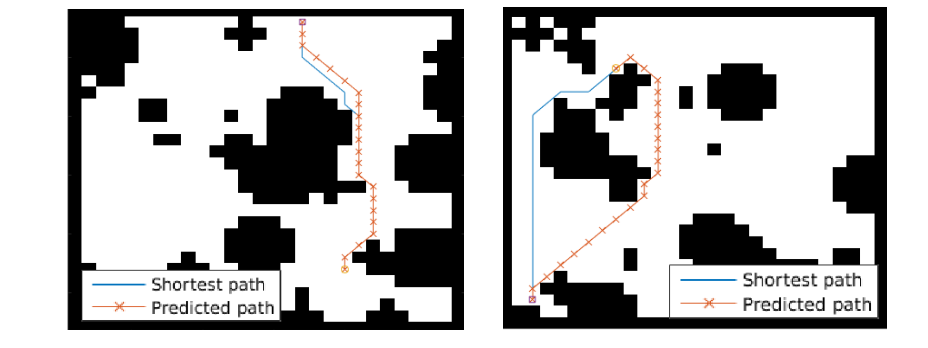
The agent gets a reward +1 in the goal state, -1 in obstacles (black), and -0.01 for each step (so that the shortest path to the goal is an optimal solution).
## VIN model
The agent is implemented in a very straight-forward manner as a single neural network trained with TRPO (Policy Gradients with a KL constraint on predictive action distributions over a batch of trajectories). So the only loss function used is to maximize expected reward, as is standard in model-free RL. However, the policy network of the agent has a very specific structure since it (internally) runs value iteration.
First, there's the core Value Iteration **(VI) Module** which runs the recurrence formula (reproducing again):

The input to this recurrence are the two arrays R (the reward array, reward for each state) and P (the dynamics array, the probabilities of transitioning to nearby states with each action), which are of course unknown to the agent, but can be predicted with neural networks as a function of the current state. This is a little funny because the networks take a _particular_ state **s** and are internally (during the forward pass) predicting the rewards and dynamics for all states and actions in the entire environment. Notice, extremely importantly and once again, that at no point are the reward and dynamics functions explicitly regressed to the observed transitions in the environment. They are just arrays of numbers that plug into value iteration recurrence module.
But anyway, once we have **R,P** arrays, in the Grid-world above due to the local connectivity, value iteration can be implemented with a repeated application of convolving **P** over **R**, as these filters effectively *diffuse* the estimated reward function (**R**) through the dynamics model (**P**), followed by max pooling across the actions. If **P** is a not a function of the state, it would simply be the filters in the Conv layer. Notice that posing this as convolution also assumes that the env dynamics are position-invariant. See the diagram below on the right: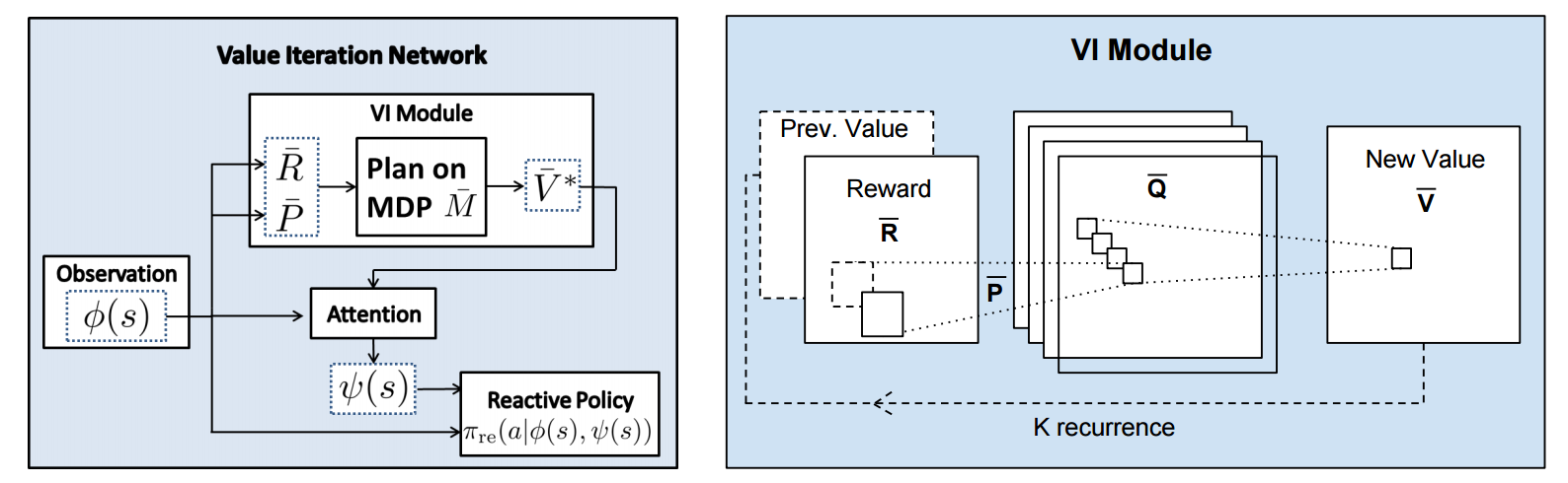
Once the array of numbers that we interpret as holding the estimated $V^*$ is computed after running **K** steps of the recurrence (K is fixed beforehand. For example for a 16x16 map it is 20, since that's a bit more than the amount of steps needed to diffuse rewards across the entire map), we "pluck out" the state-action values $Q(s,.)$ at the state the agent happens to currently be in (by an "attention" operator $\psi$), and (optionally) append these Q values to the feedforward representation of the current state $\phi(s)$, and finally predicting the action distribution.
## Experiments
**Baseline 1**: A vanilla ConvNet policy trained with TRPO. [(50 3x3 filters)\*2, 2x2 max pool, (100 3x3 filters)\*3, 2x2 max pool, FC(100), FC(4), Softmax].
**Baseline 2**: A fully convolutional network (FCN), 3 layers (with a filter that spans the whole image), of 150, 100, 10 filters. i.e. slightly different and perhaps a bit more domain-appropriate ConvNet architecture.
**Curriculum** is used during training where easier environments are trained on first. This is claimed to work better but not quantified in tables. Models are trained with TRPO, RMSProp, implemented in Theano.
Results when training on **5000** random grid-world instances (hey isn't that quite a bit low?):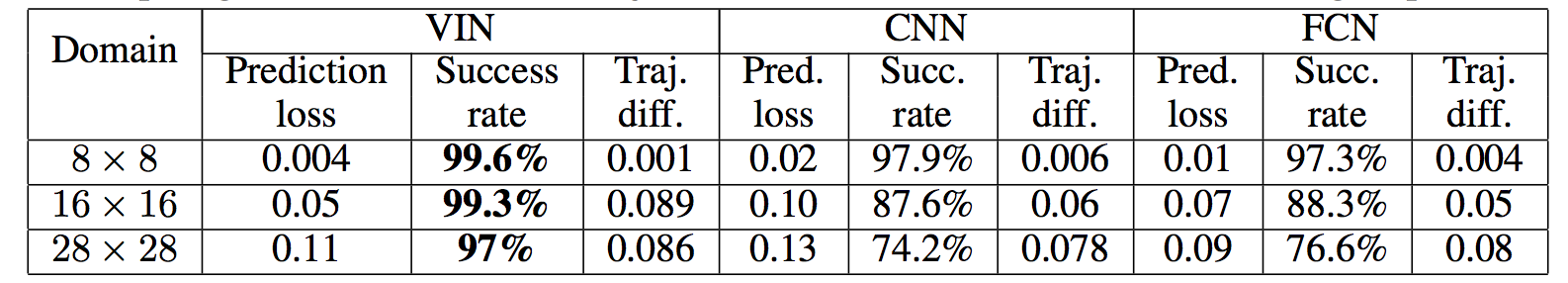
TLDR VIN generalizes better.
The authors also run the model on the **Mars Rover Navigation** dataset (wait what?), a **Continuous Control** 2D path planning dataset, and the **WebNav Challenge**, a language-based search task on a graph (of a subset of Wikipedia). Skipping these because they don't add _too_ much to the core cool idea of the paper.
## Misc
**The good**: I really like this paper because the core idea is cute (the planner is *embedded* in the policy and trained end-to-end), novel (I don't think I saw this idea executed on so far elsewhere), the paper is well-written and clear, and the supplementary materials are thorough.
**On the approach**: Significant challenges remain to make this approach more practicaly viable, but it also seems that much more exciting followup work can be done in this framework. I wish the authors discussed this more in the conclusion. In particular, it seems that one has to explicitly encode the environment connectivity structure in the internal model $\bar{M}$. How much of a problem is this and what could be done about it? Or how could we do the planning in more higher-level abstract spaces instead of the actual low-level state space of the problem? Also, it seems that a potentially nice feature of this approach is that the agent could dynamically "decide" on a reward function at runtime, and the VI module can diffuse it through the dynamics and hence do the planning. A potentially interesting outcome is that the agent could utilize this kind of computation so that an LSTM controller could learn to "emit" reward function subgoals and the VI planner computes how to meet them. A nice/clean division of labor one could hope for in principle.
**The experiments**. Unfortunately, I'm not sure why the authors preferred breadth of experiments and sacrificed depth of experiments. I would have much preferred a more in-depth analysis of the gridworld environment. For instance:
- Only 5,000 training examples are used for training, which seems very little. Presumable, the baselines get stronger as you increase the number of training examples?
- Lack of visualizations: Does the model actually learn the "correct" rewards **R** and dynamics **P**? The authors could inspect these manually and correlate them to the actual model. This would have been reaaaallllyy cool. I also wouldn't expect the model to exactly learn these, but who knows.
- How does the model compare to the baselines in the number of parameters? or FLOPS? It seems that doing VI for 30 steps at each single iteration of the algorithm should be quite expensive.
- The authors should study the performance as a function of the number of recurrences **K**. A particularly funny experiment would be K = 1, where the model would be effectively predicting **V*** directly, without planning. What happens?
- If the output of VI $\psi(s)$ is concatenated to the state parameters, are these Q values actually used? What if all the weights to these numbers are zero in the trained models?
- Why do the authors only evaluate success rate when the training criterion is expected reward?
Overall a very cute idea, well executed as a first step and well explained, with a bit of unsatisfying lack of depth in the experiments in favor of breadth that doesn't add all that much.
2 Comments
  |
