* DRAW = deep recurrent attentive writer
  * DRAW is a recurrent autoencoder for (primarily) images that uses attention mechanisms.
  * Like all autoencoders it has an encoder, a latent layer `Z` in the "middle" and a decoder.
  * Due to the recurrence, there are actually multiple autoencoders, one for each timestep (the number of timesteps is fixed).
  * DRAW has attention mechanisms which allow the model to decide where to look at in the input image ("glimpses") and where to write/draw to in the output image.
  * If the attention mechanisms are skipped, the model becomes a simple recurrent autoencoder.
  * By training the full autoencoder on a dataset and then only using the decoder, one can generate new images that look similar to the dataset images.


![DRAW Architecture](https://raw.githubusercontent.com/aleju/papers/master/neural-nets/images/DRAW_A_Recurrent_Neural_Network_for_Image_Generation__architecture.png?raw=true "DRAW Architecture")

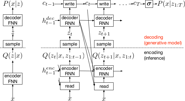
*Basic recurrent architecture of DRAW.*


### How
  * General architecture
    * The encoder-decoder-pair follows the design of variational autoencoders.
    * The latent layer follows an n-dimensional gaussian distribution. The hyperparameters of that distribution (means, standard deviations) are derived from the output of the encoder using a linear transformation.
    * Using a gaussian distribution enables the use of the reparameterization trick, which can be useful for backpropagation.
    * The decoder receives a sample drawn from that gaussian distribution.
    * While the encoder reads from the input image, the decoder writes to an image canvas (where "write" is an addition, not a replacement of the old values).
    * The model works in a fixed number of timesteps. At each timestep the encoder performs a read operation and the decoder a write operation.
    * Both the encoder and the decoder receive the previous output of the encoder.
  * Loss functions
    * The loss function of the latent layer is the KL-divergence between that layer's gaussian distribution and a prior, summed over the timesteps.
    * The loss function of the decoder is the negative log likelihood of the image given the final canvas content under a bernoulli distribution.
    * The total loss, which is optimized, is the expectation of the sum of both losses (latent layer loss, decoder loss).
  * Attention
    * The selective read attention works on image patches of varying sizes. The result size is always NxN.
    * The mechanism has the following parameters:
        * `gx`: x-axis coordinate of the center of the patch
        * `gy`: y-axis coordinate of the center of the patch
        * `delta`: Strides. The higher the strides value, the larger the read image patch.
        * `sigma`: Standard deviation. The higher the sigma value, the more blurry the extracted patch will be.
        * `gamma`: Intensity-Multiplier. Will be used on the result.
        * All of these parameters are generated using a linear transformation applied to the decoder's output.
    * The mechanism places a grid of NxN gaussians on the image. The grid is centered at `(gx, gy)`. The gaussians are `delta` pixels apart from each other and have a standard deviation of `sigma`.
    * Each gaussian is applied to the image, the center pixel is read and added to the result.


![DRAW Attention](https://raw.githubusercontent.com/aleju/papers/master/neural-nets/images/DRAW_A_Recurrent_Neural_Network_for_Image_Generation__attention.png?raw=true "DRAW Attention")

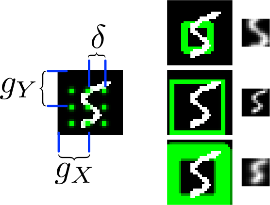
*The basic attention mechanism. (gx, gy) is the read patch center. delta is the strides. On the right: Patches with different sizes/strides and standard deviations/blurriness.*


### Results
  * Realistic looking generated images for MNIST and SVHN.
  * Structurally OK, but overall blurry images for CIFAR-10.
  * Results with attention are usually significantly better than without attention.
  * Image generation without attention starts with a blurry image and progressively sharpens it.

![DRAW SVHN Results](https://raw.githubusercontent.com/aleju/papers/master/neural-nets/images/DRAW_A_Recurrent_Neural_Network_for_Image_Generation__svhn.png?raw=true "DRAW SVHN Results")

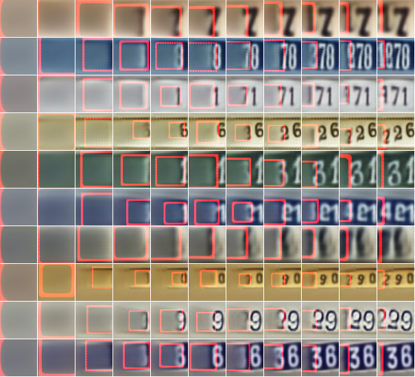
*Using DRAW with attention to generate new SVHN images.*

----------

### Rough chapter-wise notes

* 1. Introduction
  * The natural way to draw an image is in a step by step way (add some lines, then add some more, etc.).
  * Most generative neural networks however create the image in one step.
  * That removes the possibility of iterative self-correction, is hard to scale to large images and makes the image generation process dependent on a single latent distribution (input parameters).
  * The DRAW architecture generates images in multiple steps, allowing refinements/corrections.
  * DRAW is based on varational autoencoders: An encoder compresses images to codes and a decoder generates images from codes.
  * The loss function is a variational upper bound on the log-likelihood of the data.
  * DRAW uses recurrance to generate images step by step.
  * The recurrance is combined with attention via partial glimpses/foveations (i.e. the model sees only a small part of the image).
  * Attention is implemented in a differentiable way in DRAW.

* 2. The DRAW Network
  * The DRAW architecture is based on variational autoencoders:
    * Encoder: Compresses an image to latent codes, which represent the information contained in the image.
    * Decoder: Transforms the codes from the encoder to images (i.e. defines a distribution over images which is conditioned on the distribution of codes).
  * Differences to variational autoencoders:
    * Encoder and decoder are both recurrent neural networks.
    * The encoder receives the previous output of the decoder.
    * The decoder writes several times to the image array (instead of only once).
    * The encoder has an attention mechanism. It can make a decision about the read location in the input image.
    * The decoder has an attention mechanism. It can make a decision about the write location in the output image.
  * 2.1 Network architecture
    * They use LSTMs for the encoder and decoder.
    * The encoder generates a vector.
    * The decoder generates a vector.
    * The encoder receives at each time step the image and the output of the previous decoding step.
    * The hidden layer in between encoder and decoder is a distribution Q(Zt|ht^enc), which is a diagonal gaussian.
    * The mean and standard deviation of that gaussian is derived from the encoder's output vector with a linear transformation.
    * Using a gaussian instead of a bernoulli distribution enables the use of the reparameterization trick. That trick makes it straightforward to backpropagate "low variance stochastic gradients of the loss function through the latent distribution".
    * The decoder writes to an image canvas. At every timestep the vector generated by the decoder is added to that canvas.
  * 2.2 Loss function
    * The main loss function is the negative log probability: `-log D(x|ct)`, where `x` is the input image and `ct` is the final output image of the autoencoder. `D` is a bernoulli distribution if the image is binary (only 0s and 1s).
    * The model also uses a latent loss for the latent layer (between encoder and decoder). That is typical for VAEs. The loss is the KL-Divergence between Q(Zt|ht_enc) (`Zt` = latent layer, `ht_enc` = result of encoder) and a prior `P(Zt)`.
    * The full loss function is the expection value of both losses added up.
  * 2.3 Stochastic Data Generation
    * To generate images, samples can be picked from the latent layer based on a prior. These samples are then fed into the decoder. That is repeated for several timesteps until the image is finished.

* 3. Read and Write Operations
  * 3.1 Reading and writing without attention
    * Without attention, DRAW simply reads in the whole image and modifies the whole output image canvas at every timestep.
  * 3.2 Selective attention model
    * The model can decide which parts of the image to read, i.e. where to look at. These looks are called glimpses.
    * Each glimpse is defined by its center (x, y), its stride (zoom level), its gaussian variance (the higher the variance, the more blurry is the result) and a scalar multiplier (that scales the intensity of the glimpse result).
    * These parameters are calculated based on the decoder output using a linear transformation.
    * For an NxN patch/glimpse `N*N` gaussians are created and applied to the image. The center pixel of each gaussian is then used as the respective output pixel of the glimpse.
  * 3.3 Reading and writing with attention
    * Mostly the same technique from (3.2) is applied to both reading and writing.
    * The glimpse parameters are generated from the decoder output in both cases. The parameters can be different (i.e. read and write at different positions).
    * For RGB the same glimpses are applied to each channel.

* 4. Experimental results
  * They train on binary MNIST, cluttered MNIST, SVHN and CIFAR-10.
  * They then classfiy the images (cluttered MNIST) or generate new images (other datasets).
  * They say that these generated images are unique (to which degree?) and that they look realistic for MNIST and SVHN.
  * Results on CIFAR-10 are blurry.
  * They use binary crossentropy as the loss function for binary MNIST.
  * They use crossentropy as the loss function for SVHN and CIFAR-10 (color).
  * They used Adam as their optimizer.
  * 4.1 Cluttered MNIST classification
    * They classify images of cluttered MNIST. To do that, they use an LSTM that performs N read-glimpses and then classifies via a softmax layer.
    * Their model's error rate is significantly below a previous non-differentiable attention based model.
    * Performing more glimpses seems to decrease the error rate further.
  * 4.2 MNIST generation
    * They generate binary MNIST images using only the decoder.
    * DRAW without attention seems to perform similarly to previous models.
    * DRAW with attention seems to perform significantly better than previous models.
    * DRAW without attention progressively sharpens images.
    * DRAW with attention draws lines by tracing them.
  * 4.3 MNIST generation with two digits
    * They created a dataset of 60x60 images, each of them containing two random 28x28 MNIST images.
    * They then generated new images using only the decoder.
    * DRAW learned to do that.
    * Using attention, the model usually first drew one digit then the other.
  * 4.4 Street view house number generation
    * They generate SVHN images using only the decoder.
    * Results look quite realistic.
  * 4.5 Generating CIFAR images
    * They generate CIFAR-10 images using only the decoder.
    * Results follow roughly the structure of CIFAR-images, but look blurry.

Prior to this paper, most methods that used machine learning to generate molecular blueprints did so using SMILES representations - a string format with characters representing different atoms and bond types. This preference came about because ML had existing methods for generating strings that could be built on for generating SMILES (a particular syntax of string). However, an arguably more accurate and fundamental way of representing molecules is as graphs (with atoms as nodes and bonds as edges). Dealing with molecules as graphs avoids the problem of a given molecule having many potential SMILES representations (because there's no canonical atom to start working your way around the molecule on), and, hopefully, would have an inductive bias that somewhat more closely matches the actual biomechanical interactions within a molecule. 

One way you could imagine generating a graph structure is by adding on single components (atoms or bonds) at a time. However, the authors of this paper argue that this approach is harder to constrain to only construct valid molecular graphs, since, in the course of sampling out a molecule, you'd have to go through intermediate stages that you expect to be invalid (for example, bonds with no attached atoms), making it hard to add in explicit validity checks. The alternate approach proposed here works as follows: 

- Atoms within molecules are grouped into valid substructures, based on a combination of biologically-motivated rules (like treating aromatic rings as a single substructure) and computational heuristics. For the purpose of this paper, substructures are generally either 1) a ring, 2) two particular atoms on either end of a bond, or 3) a "tail" with a bond and an atom. Importantly, these substructures are designed to be overlapping - if you had a N bonded with O, and then O with C (this example are entirely made up, and I expect chemically incoherent), then you could have "N-O" as one substructure, and "O-C" as another.

https://i.imgur.com/yGzRPjT.png

- Using these substructures (or clusters), you can form a simplified representation of a molecule, as a connected, non-cyclic junction tree of clusters connected together. This doesn't give you all the information you'd need to construct the molecule - since there could be multiple different ways, on a molecular level, to connect two substructures, but it does give a blueprint of what the molecule will look like.
- Given these two representations, the paper proposes a two-step encoding and decoding process. For a given molecule, we encode both the full molecular graph and the simplified junction tree, getting out vectors Zg and Zt respectively.
- The first step of decoding generates a tree given the Zt representation. This generation process works via graph message-passing, taking in the Zt vector in addition to whatever part of the tree exists, and predicting a probability for whether that node has a child, and, if it exists, a probability for what cluster is at that child node. Given this parametrized set of probabilities, we can calculate the probability of the junction tree representation of whatever ground truth molecule we're decoding, and train the tree decoder to increase that model likelihood. (Importantly, although we frame this step as "reconstruction," during training, we're not actually sampling discrete nodes and edges, because we couldn't backprop through that, we're just defining a probability distribution and trying to increase the probability of our real data under it).
- The second step of decoding takes in a tree - which at this point is a set of cluster labels with connections specified between one another - as well as the Zg vector, and generates a full, atom-level graph. This is done by enumerating all the ways that two substructures could be attached (this number is typically small, ≤4), and learning a parametrized function that scores each possible type of connection, based on the full tree "blueprint", the Zg embedding, and the molecule that has been generated so far.
- When you want to sample a new molecule, you can draw a sample from the prior distributions of Zg and Zt, and run the decoding process in a sampling mode, actually making discrete draws from the distributions given by your model

https://i.imgur.com/QdSY25u.png

The authors perform three empirical tests: ability to successfully sample-reconstruct a given molecule, ability to optimize for a desired chemical property by finding a Z that scores high on that property according to an auxiliary predictive model, and ability to optimize for a property while staying within a given similarity radius to an original anchor molecule. The Junction Tree approach outperforms on all three tasks. On reconstruction, it matches the best alternative method on reconstruction reliability, but with 100% valid molecules, rather than 43.5% on the competing method. 

Overall, I found this paper really enjoyable and satisfying to read. Occasionally, ML-for-bio papers err on the side of too little domain thought (just throwing the most generic-for-images model structure at a problem), or too little machine learning thought (take hand-designed features and throw them at a whole range of models), where I think this one struck a nice balance of some amount of domain knowledge (around what makes for valid substructures) but embedded in a complex and thoughtfully designed neural network framework.

The paper discusses the idea of using BERT pre-trained network in bio-medical domain NLP tasks. It lays a path for future applications of Bert in different business verticals. Sharing some points from the review article I wrote on BioBERT on medium (https://medium.com/@raghudeep/biobert-insights-b4c66fde8fa7).

The major contribution is a pre-trained bio-medical language representation model for various bio-medical text mining tasks. Tasks such as NER from Bio-medical data, relation extraction, question & answer in the biomedical field.

For pretraining the model, authors have used a combination of general & medical corpora, which has shown interesting results. They have compared the results of all their combinations.

Google's team developed scheduled sampling as an alternative training procedure to fit RNNs, and they used it in their competition-winning method for image captioning. While I can't argue with the empirical results (so I won't), I was a bit skeptical about the technique at a fundamental level, so I decided to do a bit of math that resulted in this blog post.

Overall, I have a suspicion that scheduled sampling is a flawed objective function for unsupervised/generative modelling, and I want to use this post to explain why I think so. I hope the comments section will work this time so people can comment and argue otherwise. Please also shoot me an email if you have more to say.

#### Summary of this note

- I have a critical look at scheduled sampling as objective function for training RNNs
- I show it can lead to pathologies where the RNN learns marginal instead of conditional distributions
- I explain why I think adversarial training/generative moment matching offers a better alternative
- Lastly, I include a paragraph in which I apologise for being a di*k again.

#### Strictly proper scoring rules

I've mentioned scoring rules on this blog many times, and my PhD thesis was about them, so saying I'm obsessed with this topic would be a valid observation. But this is important stuff, particularly for unsupervised learning, and particularly as a framework to think about hard concepts like overfitting in generative models.

Scoring rules are essentially loss functions for probabilistic models/forecasts. A scoring rule $$S(x,Q)$$ simply measures how bad a probabilistic forecast $Q$ for a variable is in the light of actual observation $x$. In this notation, lower is better. A scoring rule is called strictly proper, if for any $P$, the following holds:

$$\underset{Q}{\operatorname{argmax}} \mathbb{E}_{x\sim P}S(x,Q) = P$$

In other words, if you repeatedly sample observations from some true underlying distribution $P$, then the model $Q$ which minimises expected score is $P$. This means that the scoring rule cannot be fooled and that minimising the expected score yields a consistent estimator for $P$. Because I mention consistency, people may dismiss this as a learning theory argument, but it is not. If you are a Bayesian or a deep learning person with no interest in consistency, a scoring rule being strictly proper simply means that it is safe to use it as a loss function. Anything that's not strictly proper is weird and wrong, it will lead to learning the wrong thing.

This concept is central in unsupervised learning and generative modelling. Unsupervised learning is all about modelling the probability distribution of data, so it's essential that we have loss functions that can measure the discrepancy between our model $Q$, and the true data distribution $P$ in a consistent way.

#### log-likelihood

One of the most frequently used strictly proper scoring rule is the logarithmic score:

$$S(x,Q) = - \log Q(x)$$

This quantity is also known as the negative log-likelihood. Minimising the expected score in an i.i.d scenario yields maximum likelihood estimation, which is known to be a consistent estimator and has nice properties.

Often, the likelihood is impossible to evaluate. Luckily, it is not the only strictly proper scoring rule. In the context of generative models people have used the pseudolikelihood, score matching and moment matching, all of which are examples of strictly proper scoring rules.

To recap, any learning method that corresponds to minimising a strictly proper scoring rule is fine, everything else can go horribly wrong, even if we feed it infinite data, it might just learn the wrong thing.

#### Scheduled Sampling

After successfully establishing myself as a proper-scoring-rule-nazi, let's talk about scheduled sampling (SS). I don't have a lot of space explaining SS in great detail here, only the basic idea. I encourage everyone to read the paper and Hugo's summary above.

SS is a new method to train recurrent neural networks(RNNs) to model sequences. I will use character-by-character models of text as an example. Typically, when you train an RNN, you aim to minimise the log predictive likelihood in predicting the next character in each training sentence, given the prefix string of previous characters. This can be thought of as a special case of maximum likelihood learning, and is all fine, you can actually do this properly without approximations.

After training, you use the RNN to generate sample sentences in a recursive fashion: assuming you've already generated $n$ characters, you feed that prefix into the RNN, and ask it to predict the $n+1$st character. The $n+1$st character is then added to the prefix to predict the $n+2$th character, and so on.

The authors say there is a disconnect between how the model is trained (it's always fed real data) and how it's used (it's always fed synthetic data generated by itself). This, they argue, leads to the RNN being unable to recover from its own mistakes early on in the sentence.

To address this, the authors propose an alternative training strategy, where every once in a while, the network is given its own synthetic data instead of real data at training time. More specifically, for each character in the training sentences, we flip a coin to decide whether we feed the character from the real training sentence, or whether to feed the model's own prediction as to what that character would have been. The authors claim this makes the model more robust to recovering from mistakes, which is probably true.

As far as I'm concerned, I'm happy as long as the new training procedure corresponds to a strictly proper scoring rule. But in this case, I have a strong feeling that it does not.

#### case study: sequence of two variables

For sake of simplicity, let's consider using scheduled sampling to learn the joint distribution of a sequence of just two random variables. This is probably the simplest (shortest) time series I can think of. So SS in this case works as follows: For each datapoint train the network to predict the real $x_1$. Then we flip a coin to decide whether to keep $x_1$ from the datapoint, or to replace it with a sample from the model $Q_{x_1}$. Then we train $Q_{x_2\vert x_1}$ on the $(x_1,x_2)$ pair obtained this way.

The scoring rule for selective sampling looks something like this:

$$ S(Q_{x_1,x_2},(x_1,x_2)) = - (1 - \epsilon) [ \mathbb{E}_{z \sim Q_{x_1}} \log Q_{x_2 \vert x_1}(x_2 \vert z) + \log Q_{x_1}(x_1)] - \epsilon \log Q_{x_2 , x_1}(x_1,x_2),$$

where $\epsilon$ is the probability with wich the true $x_1$ is used.

The authors suggest starting training with $\epsilon=1$ and annealing it so that by the end of the training $\epsilon=0$. So as far as the eventual optimum of SS is concerned, we only have to focus on what the first term of the scoring rule does. The second term is the good old log-likelihood so we know that part works.

After some math, one can show that scheduled sampling with a fixed $\epsilon$ minimises the following divergence between the true $P$ and the model $Q$:

$$D_{SS}[P\|Q] = KL[P_{x_1}\|Q_{x_1}] + (1-\epsilon) \mathbb{E}_{z\sim Q_{x_1}} KL[P_{x_2}\|Q_{x_2\vert x_1=z}] + \epsilon KL[P_{x_2\vert x_1}\|Q_{x_2\vert x_1}]$$

Now, if $\epsilon=1$, we recover the Kullback-Leibler divergence between the joint $P_{x_1,x_2}$ and $Q_{x_1,x_2}$, which is what we expect as it corresponds to maximum likelihood estimation. However, as $\epsilon$ is annealed to $0$, the objective function is somewhat strange, whereby the conditional distribution $Q_{x_2\vert x_1}$ is pushed to model the marginal distribution $P_{x_2}$, instead of $P_{x_2\vert x_1}$ as one would expect. One can therefore see that the factorised $Q^{*} = P_{x_1}P_{x_2}$ minimises this objective function.

#### what this means for text modeling

Extrapolating from the two variable case to longer sequences, one can see that the scheduled sampling objective would fail if minimised properly until convergence. Consider the case when the $\epsilon\approx 0$ stage is reached in the annealing schedule. Now consider what the RNN has to do to predict the $n$th character in a string during training. It is fed a random prefix string that was generated by itself but never seen any real data. Then the RNN has to give a probabilistic forecast of what the $n$th character in the training sentence is, having seen none of the previous characters in the sentence.

The optimal model that minimises this objective would completely ignore all the characters in the sentence so far, but keep a simple linear counter that indexes where it is within the sentence. Then it would emit a character from an index-specific marginal distribution of characters. This is the equivalent of the factorised trivial solution above.

Yes, such a model would be better at "recovering from its own mistakes", because at every character it would start independently from what it has generated so far. But this is at the cost of paying no attention whatsoever as to what the prefix of the sentence was. I believe the reason why this trivial behaviour was not observed in the paper is that the authors did not run the optimisation until convergence, and did not implement the full gradient of the objective function, as they discuss in the paper.

#### Constructive part of criticism

#### What to do instead of SS?

So the observed problem was that RNNs trained via maximum likelihood are unable to recover from their own mistakes early on in a sentence, when they are used to generate.

`The main reason for the observed problem is that the log-likelihood is a local scoring rule`

The local property of scoring rules means that at training time we only ever evaluate the model $Q$ on actually observed datapoints. So if the RNN is faced with a prefix subsequence that was not in the dataset, God knows what it's going to complete that sentence with.

The proper (shall I say strictly proper) way to fix this issue is to use 

When running an application in the cloud, users have to trust (i) the cloud provider's software, (ii) the cloud provider's staff, and (iii) law enforcement with the ability to access user data. Intel SGX partially solves this problem by allowing users to run small portions of program on remote servers with guarantees of confidentiality and integrity. Haven leverages SGX and Drawbridge to run entire legacy programs with shielded execution.

Haven assumes a very strong adversary which has access to all the system's software and most of the system's hardware. Only the processor and SGX hardware is trusted. Haven provides confidentiality and integrity, but not availability. It also does not prevent side-channel attacks.

There are two main challenges that Haven's design addresses. First, most programs are written assuming a benevolent host. This leads to Iago attacks in which the OS subverts the application by exploiting its assumptions about the OS. Haven must operate correctly despite a malicious host. To do so, Haven uses a library operation system LibOS that is part of a Windows sandboxing framework called Drawbridge. LibOS implements a full OS API using only a few core host OS primitives. These core host OS primitives are used in a defensive way. A shield module sits below LibOS and takes great care to ensure that LibOS is not susceptible to Iago attacks. The user's application, LibOS, and the shield module are all run in an SGX enclave.

Second, Haven aims to run unmodified binaries which were not written with knowledge of SGX. Real world applications allocate memory, load and run code dynamically, etc. Many of these things are not supported by SGX, so Haven (a) emulated them and (b) got the SGX specification revised to address them.

Haven also implements an in-enclave encrypted file system in which only the root and leaf pages need to be written to stable storage. As of publication, however, Haven did not fully implement this feature. Haven is susceptible to replay attacks.

Haven was evaluated by running Microsoft SQL Server and Apache HTTP Server.