This is heavily derived from the top voted summary above, but I had to review this paper for a lab meeting so I expanded on it a bit. I hope this doesn't offend anyone, but this should be, at worst, redundant to the summary above.

This paper has two parts: five recommended techniques for training GANs and
a thorough evaluation with visual Turing tests and semi-supervised tasks.
That is more concrete than the feature extraction and visualisation in, for
example, Radford's [DCGAN paper][dcgan].

### Feature Matching

Problem: instability from overtraining on the current discriminator.
Intuition is that the discriminator will have learnt the kind of useful
representation we see in deep image models, and there is more information
available by matching those than the single classifier output.

Solution: Match activations at some hidden with an L2 loss. This is
the same as the "content" loss in the [neural style paper][style]:

$$
\newcommand{\aB}{\mathbf{a}}
\newcommand{\bB}{\mathbf{b}}
\newcommand{\cB}{\mathbf{c}}
\newcommand{\dB}{\mathbf{d}}
\newcommand{\eB}{\mathbf{e}}
\newcommand{\fB}{\mathbf{f}}
\newcommand{\gB}{\mathbf{g}}
\newcommand{\hB}{\mathbf{h}}
\newcommand{\iB}{\mathbf{i}}
\newcommand{\jB}{\mathbf{j}}
\newcommand{\kB}{\mathbf{k}}
\newcommand{\lB}{\mathbf{l}}
\newcommand{\mB}{\mathbf{m}}
\newcommand{\nB}{\mathbf{n}}
\newcommand{\oB}{\mathbf{o}}
\newcommand{\pB}{\mathbf{p}}
\newcommand{\qB}{\mathbf{q}}
\newcommand{\rB}{\mathbf{r}}
\newcommand{\sB}{\mathbf{s}}
\newcommand{\tB}{\mathbf{t}}
\newcommand{\uB}{\mathbf{u}}
\newcommand{\vB}{\mathbf{v}}
\newcommand{\wB}{\mathbf{w}}
\newcommand{\xB}{\mathbf{x}}
\newcommand{\yB}{\mathbf{y}}
\newcommand{\zB}{\mathbf{z}}
\newcommand{\Exp}{\mathbb{E}}
|| \Exp_{\xB \sim p_{\text{data}}} \fB (\xB) - \Exp_{\zB \sim p_{\zB}(\zB)} \fB (G(\zB)) ||_2^2
$$

Where $\fB (\xB)$ and $\fB (\zB)$ are the activations in some hidden layer
corresponding to either a real or generated image.

### Minibatch Discrimination

Problem: generators like to collapse to a single mode (ie just generate a
single image), because it's a decent local optimum.

Solution: make sure the discriminator can look at samples in combination,
so it will know if it's getting the same (or similar) images more easily.
Just give the discriminator features that tell it about the distance of
each image to other images in the same batch. The diagram in the paper
describes this best.

They mention this tensor $T$ in the paper, but don't really explain what it
is. In [the code][mbcode], it appears to be basically a weight matrix,
which means that it is also learnt as part of the discriminator.

### Historical Averaging

Problem: no guarantee with gradient descent that a two player game like
this won't go into extended orbits.

Solution: encourage parameters to revert to their historical mean, with an
L2 penalty:

$$
\newcommand{\thetaB}{\boldsymbol{\theta}}
|| \thetaB - \frac{1}{t} \sum_{i=1}^t \thetaB[i] ||^2
$$

Orbits are penalised by always being far from their mean, and this is
supposed to correspond to a "fictitious play" algorithm. I'm not sure if
that's true, but maybe?

### One-sided label smoothing

Problem: vulnerability of discriminator to adversarial examples? (Not
explicitly stated).

Solution: replace positive (ie probability that a sample is real?) labels
with a target _smaller than 1_.

### Virtual Batch Normalisation

Problem: batch normalisation is highly variable, as it is based on
statistics of the current minibatch (enough so that you can sometimes avoid
using dropout if you're using batchnorm).

Solution: for every minibatch, use the statistics gathered from a
_reference minibatch_ for your batch normalisation. For every minibatch,
you'll have to first propagate through the reference minibatch with your
current parameter settings, but then you can use the statistics you gather
by doing this for the minibatch you're actually going to use for training.

_Interesting sidenote_: in the [code][impcode], they are actually using
[weight normalization][weightnorm] instead of batchnorm (not in all cases).
Probably because both papers have Tim Salimans as first author.

### Assessing Image Quality

Problem: noisy labelling from mechanical turk.

Solution: aim for low entropy conditional categorical distribution when
labelling samples with Google's inception model. The inception model gives
you $p(y|\xB)$, so you want to maximise:

$$
\Exp_{\xB} KL (p(y|\xB)||p(y))
$$

Then they exponentiate the resulting value for no real reason, just to make
values easier to compare. Since they say this matches human judgement in
their experiments, this means we can all start using this measure and just
cite this paper!

### Semi-supervised Learning

Problem: standard semi-supervised, we have some data that is labelled and
some that isn't, how to learn a conditional model that will give us
$p(y|\xB)$.

Solution: make "generated" a class in your classification problem. Now you
can put generated samples into your dataset, but even better you can
produce a loss on unlabeled samples that you just _don't want them to be
labeled as "generated"_. So we end up with the following two losses for
supervised and unsupervised data:

$$
L_{\text{supervised}} = - \Exp_{\xB,y \sim p_{\text{data}} (\xB, y)} \log p_{\text{model}} (y | \xB, y < K + 1)
$$

$$
L_{\text{unsupervised}} = - \{ \Exp_{\xB \sim p_{\text{data}} (\xB)} \log [
1- p_{\text{model}} (y = K+1 | \xB) ] + \Exp_{\xB \sim G}\log [
p_{\text{model}} (y=K+1 | \xB)] \}
$$

With this method, and using feature matching but _not minibatch
discrimination_, they show SOTA results for semi-supervised learning on
MNIST, SVHN and CIFAR-10.

[mbcode]: https://github.com/openai/improved-gan/blob/master/mnist_svhn_cifar10/nn.py#L132-L170
[impcode]: https://github.com/openai/improved-gan/blob/master/mnist_svhn_cifar10/nn.py#L45-L91
[weightnorm]: https://arxiv.org/abs/1602.07868
[short]: http://www.shortscience.org/paper?bibtexKey=journals/corr/SalimansGZCRC16#udibr
[improved]: https://arxiv.org/abs/1606.03498
[dcgan]: https://arxiv.org/abs/1511.06434
[style]: https://arxiv.org/abs/1508.06576

This paper argues for the use of normalizing flows - a way of building up new probability distributions by applying multiple sets of invertible transformations to existing distributions - as a way of building more flexible variational inference models. 

The central premise of a variational autoencoder is that of learning an approximation to the posterior distribution of latent variables - p(z|x) - and parameterizing that distribution according to values produced by a neural network. In typical practice, this has meant that VAEs are limited in terms of the complexity of latent variable distributions they can encode, since using an analytically specified distribution tends to limit you to simpler distributional shapes - Gaussians, uniform, and the like. Normalizing flows are here proposed as a way to allow for the model to learn more complex forms of posterior distribution. 

Normalizing flows work off of a fairly simple intuition: if you take samples from a distribution p(x), and then apply a function f(x) to each x in that sample, you can calculate the expected value of your new distribution f(x) by calculating the expectation of f(x) under the old distribution p(x). That is to say: 
https://i.imgur.com/NStm7zN.png
This mathematical transformation has a pretty delightful name - The Law of the Unconscious Statistician - that came from the fact that so many statisticians just treated this identity as a definitional fact, rather than something actually in need of proving (I very much fall into this bucket as well). The implication of this is that if you apply many transformations in sequence to the draws from some simple distribution, you can work with that distribution without explicitly knowing its analytical formulation, just by being able to evaluate - and, importantly - invert the function. The ability to invert the function is key, because of the way you calculate the derivative: by taking the inverse of the determinant of the derivative of your function f(z) with respect to z. (Note here that q(z) is the original distribution you sampled under, and q’(z) is the implicit density you’re trying to estimate, after your function has been applied). 

https://i.imgur.com/8LmA0rc.png

Combining these ideas together: a variational flow autoencoder works by having an encoder network define the parameters of a simple distribution (Gaussian or Uniform), and then running the samples from that distribution through a series of k transformation layers. This final transformed density over z is then given to the decoder to work with. Some important limitations are in place here, the most salient of which is that in order to calculate derivatives, you have to be able to calculate the determinant of the derivative of a given transformation. Due to this constraint, the paper only tests a few transformations where this is easy to calculate analytically - the planar transformation and radial transformation. If you think about transformations of density functions as fundamentally stretching or compressing regions of density, the planar transformation works by stretching along an axis perpendicular to some parametrically defined plane, and the radial transformation works by stretching outward in a radial way around some parametrically defined point. Even though these transformations are individually fairly simple, when combined, they can give you a lot more flexibility in distributional space than a simple Gaussian or Uniform could. 

https://i.imgur.com/Xf8HgHl.png

Hein and Andriushchenko give a intuitive bound on the robustness of neural networks based on the local Lipschitz constant. With robustness, the authors refer a small $\epsilon$-ball around each sample; this ball is supposed to describe the region where the neural network predicts a constant class. This means that adversarial examples have to compute changes large enough to leave these robust areas. Larger $\epsilon$-balls imply higher robustness to adversarial examples.

When considering a single example $x$, and a classifier $f = (f_1, \ldots, f_K)^T$ (i.e. in a multi-class setting), the bound can be stated as follows. For $q$ and $p$ such that $\frac{1}{q} + \frac{1}{p} = 1$ and $c$ being the class predicted for $x$, the it holds

$x = \arg\max_j f_j(x + \delta)$

for all $\delta$ with

$\|\delta\|_p \leq \max_{R > 0}\min \left\{\min_{j \neq c} \frac{f_c(x) – f_j(x)}{\max_{y \in B_p(x, R)} \|\nabla f_c(y) - \nabla f_j(y)\|_q}, R\right\}$.

Here, $B_p(x, R)$ describes the $R$-ball around $x$ measured using the $p$-norm. Based on the local Lipschitz constant (in the denominator), the bound essentially measures how far we can deviate from the sample $x$ (measured in the $p$-norm) until $f_j(x) > f_c(x)$ for some $j \neq c$. The higher the local Lipschitz constant, the smaller deviations are allowed, i.e. adversarial examples are easier to find. Note that the bound also depends on the confidence, i.e. the edge  $f_c(x)$ has in comparison to all other $f_j(x)$.

In the remaining paper, the authors also provide bounds for simple classifiers including linear classifiers, kernel methods and two-layer perceptrons (i.e. one hidden layer). For the latter, they also propose a new type of regularization called cross-Lipschitz regularization:

$P(f) = \frac{1}{nK^2} \sum_{i = 1}^n \sum_{l,m = 1}^K \|\nabla f_l(x_i) - \nabla f_m(x_i)\|_2^2$.

This regularization term is intended to reduce the Lipschitz constant locally around training examples. They show experimental results using this regularization on MNIST and CIFAR, see the paper for details.

Also view this summary at [davidstutz.de](https://davidstutz.de/category/reading/).

### What is BN:
  * Batch Normalization (BN) is a normalization method/layer for neural networks.
  * Usually inputs to neural networks are normalized to either the range of [0, 1] or [-1, 1] or to mean=0 and variance=1. The latter is called *Whitening*.
  * BN essentially performs Whitening to the intermediate layers of the networks.

### How its calculated:
  * The basic formula is $x^* = (x - E[x]) / \sqrt{\text{var}(x)}$, where $x^*$ is the new value of a single component, $E[x]$ is its mean within a batch and `var(x)` is its variance within a batch.
  * BN extends that formula further to $x^{**} = gamma * x^* +$ beta, where $x^{**}$ is the final normalized value. `gamma` and `beta` are learned per layer. They make sure that BN can learn the identity function, which is needed in a few cases.
  * For convolutions, every layer/filter/kernel is normalized on its own (linear layer: each neuron/node/component). That means that every generated value ("pixel") is treated as an example. If we have a batch size of N and the image generated by the convolution has width=P and height=Q, we would calculate the mean (E) over `N*P*Q` examples (same for the variance).

### Theoretical effects:
  * BN reduces *Covariate Shift*. That is the change in distribution of activation of a component. By using BN, each neuron's activation becomes (more or less) a gaussian distribution, i.e. its usually not active, sometimes a bit active, rare very active.
  * Covariate Shift is undesirable, because the later layers have to keep adapting to the change of the type of distribution (instead of just to new distribution parameters, e.g. new mean and variance values for gaussian distributions).
  * BN reduces effects of exploding and vanishing gradients, because every becomes roughly normal distributed. Without BN, low activations of one layer can lead to lower activations in the next layer, and then even lower ones in the next layer and so on.

### Practical effects:
  * BN reduces training times. (Because of less Covariate Shift, less exploding/vanishing gradients.)
  * BN reduces demand for regularization, e.g. dropout or L2 norm. (Because the means and variances are calculated over batches and therefore every normalized value depends on the current batch. I.e. the network can no longer just memorize values and their correct answers.)
  * BN allows higher learning rates. (Because of less danger of exploding/vanishing gradients.)
  * BN enables training with saturating nonlinearities in deep networks, e.g. sigmoid. (Because the normalization prevents them from getting stuck in saturating ranges, e.g. very high/low values for sigmoid.)


![MNIST and neuron activations](https://raw.githubusercontent.com/aleju/papers/master/neural-nets/images/Batch_Normalization__performance_and_activations.png?raw=true "MNIST and neuron activations")

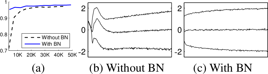
*BN applied to MNIST (a), and activations of a randomly selected neuron over time (b, c), where the middle line is the median activation, the top line is the 15th percentile and the bottom line is the 85th percentile.*

-------------------------

### Rough chapter-wise notes

* (2) Towards Reducing Covariate Shift
  * Batch Normalization (*BN*) is a special normalization method for neural networks.
  * In neural networks, the inputs to each layer depend on the outputs of all previous layers.
  * The distributions of these outputs can change during the training. Such a change is called a *covariate shift*.
  * If the distributions stayed the same, it would simplify the training. Then only the parameters would have to be readjusted continuously (e.g. mean and variance for normal distributions).
  * If using sigmoid activations, it can happen that one unit saturates (very high/low values). That is undesired as it leads to vanishing gradients for all units below in the network.
  * BN fixes the means and variances of layer inputs to specific values (zero mean, unit variance).
  * That accomplishes:
    * No more covariate shift.
    * Fixes problems with vanishing gradients due to saturation.
  * Effects:
    * Networks learn faster. (As they don't have to adjust to covariate shift any more.)
    * Optimizes gradient flow in the network. (As the gradient becomes less dependent on the scale of the parameters and their initial values.)
    * Higher learning rates are possible. (Optimized gradient flow reduces risk of divergence.)
    * Saturating nonlinearities can be safely used. (Optimized gradient flow prevents the network from getting stuck in saturated modes.)
    * BN reduces the need for dropout. (As it has a regularizing effect.)
  * How BN works:
    * BN normalizes layer inputs to zero mean and unit variance. That is called *whitening*.
    * Naive method: Train on a batch. Update model parameters. Then normalize. Doesn't work: Leads to exploding biases while distribution parameters (mean, variance) don't change.
    * A proper method has to include the current example *and* all previous examples in the normalization step.
    * This leads to calculating in covariance matrix and its inverse square root. That's expensive. The authors found a faster way.

* (3) Normalization via Mini-Batch Statistics
  * Each feature (component) is normalized individually. (Due to cost, differentiability.)
  * Normalization according to: `componentNormalizedValue = (componentOldValue - E[component]) / sqrt(Var(component))`
  * Normalizing each component can reduce the expressitivity of nonlinearities. Hence the formula is changed so that it can also learn the identiy function.
  * Full formula: `newValue = gamma * componentNormalizedValue + beta` (gamma and beta learned per component)
  * E and Var are estimated for each mini batch.
  * BN is fully differentiable. Formulas for gradients/backpropagation are at the end of chapter 3 (page 4, left).

* (3.1) Training and Inference with Batch-Normalized Networks
  * During test time, E and Var of each component can be estimated using all examples or alternatively with moving averages estimated during training.
  * During test time, the BN formulas can be simplified to a single linear transformation.

* (3.2) Batch-Normalized Convolutional Networks
  * Authors recommend to place BN layers after linear/fully-connected layers and before the ninlinearities.
  * They argue that the linear layers have a better distribution that is more likely to be similar to a gaussian.
  * Placing BN after the nonlinearity would also not eliminate covariate shift (for some reason).
  * Learning a separate bias isn't necessary as BN's formula already contains a bias-like term (beta).
  * For convolutions they apply BN equally to all features on a feature map. That creates effective batch sizes of m\*pq, where m is the number of examples in the batch and p q are the feature map dimensions (height, width). BN for linear layers has a batch size of m.
  * gamma and beta are then learned per feature map, not per single pixel. (Linear layers: Per neuron.)

* (3.3) Batch Normalization enables higher learning rates
  * BN normalizes activations.
  * Result: Changes to early layers don't amplify towards the end.
  * BN makes it less likely to get stuck in the saturating parts of nonlinearities.
  * BN makes training more resilient to parameter scales.
  * Usually, large learning rates cannot be used as they tend to scale up parameters. Then any change to a parameter amplifies through the network and can lead to gradient explosions.
  * With BN gradients actually go down as parameters increase. Therefore, higher learning rates can be used.
  * (something about singular values and the Jacobian)

* (3.4) Batch Normalization regularizes the model
  * Usually: Examples are seen on their own by the network.
  * With BN: Examples are seen in conjunction with other examples (mean, variance).
  * Result: Network can't easily memorize the examples any more.
  * Effect: BN has a regularizing effect. Dropout can be removed or decreased in strength.

* (4) Experiments
* (4.1) Activations over time
** They tested BN on MNIST with a 100x100x10 network. (One network with BN before each nonlinearity, another network without BN for comparison.)
** Batch Size was 60.
** The network with BN learned faster. Activations of neurons (their means and variances over several examples) seemed to be more consistent during training.
** Generalization of the BN network seemed to be better.

* (4.2) ImageNet classification
** They applied BN to the Inception network.
** Batch Size was 32.
** During training they used (compared to original Inception training) a higher learning rate with more decay, no dropout, less L2, no local response normalization and less distortion/augmentation.
** They shuffle the data during training (i.e. each batch contains different examples).
** Depending on the learning rate, they either achieve the same accuracy (as in the non-BN network) in 14 times fewer steps (5x learning rate) or a higher accuracy in 5 times fewer steps (30x learning rate).
** BN enables training of Inception networks with sigmoid units (still a bit lower accuracy than ReLU).
** An ensemble of 6 Inception networks with BN achieved better accuracy than the previously best network for ImageNet.

* (5) Conclusion
** BN is similar to a normalization layer suggested by Gülcehre and Bengio. However, they applied it to the outputs of nonlinearities.
** They also didn't have the beta and gamma parameters (i.e. their normalization could not learn the identity function).

Abbasi and Gagné propose explicit but natural out-distribution training as defense against adversarial examples. Specifically, as also illustrated on the toy dataset in Figure 1, they argue that networks commonly produce high-confident predictions in regions that are clearly outside of the data manifold (i.e., the training data distribution). As mitigation strategy, the authors propose to explicitly train on out-of-distribution data, allowing the network to additionally classify this data as “dustbin” data. On MNIST, for example, this data comes from NotMNIST, a dataset of letters A-J – on CIFA-10, this data could be CIFAR-100. Experiments show that this out-of-distribution training allow networks to identify adversarial examples as “dustbin” and thus improve robustness.

https://i.imgur.com/nUSDZay.png
Figure 1: Illustration of a naive model versus an augmented model, i.e., trained on out-of-distribution data, on a toy dataset (left) and on MNIST (right).

Also find this summary at [davidstutz.de](https://davidstutz.de/category/reading/).